Download
1 / 43
480 likes | 837 Vues
Hashing & Hash Tables. 1. 1. 1. 1. 1. Overview. Hash Table Data Structure : Purpose To support insertion, deletion and search in average-case constant time Assumption: Order of elements irrelevant

E N D
Hashing & Hash Tables Cpt S 223. School of EECS, WSU 1 1 1 1 1
Overview • Hash Table Data Structure : Purpose • To support insertion, deletion and search in average-case constant time • Assumption: Order of elements irrelevant • ==> data structure *not* useful for if you want to maintain and retrieve some kind of an order of the elements • Hash function • Hash[ “string key”] ==> integer value • Hash table ADT • Implementations, Analysis, Applications Cpt S 223. School of EECS, WSU 2 2 2 2
key value Hash index h(“john”) “john” TableSize key Hash function How to determine … ? Hash table: Main components Hash table(implemented as a vector) Cpt S 223. School of EECS, WSU
Hash Table Operations Hash function Hash key • Insert • T [h(“john”)] = <“john”,25000> • Delete • T [h(“john”)] = NULL • Search • T [h(“john”)] returns the element hashed for “john” Data record • What happens if h(“john”) == h(“joe”) ? • “collision” Cpt S 223. School of EECS, WSU
Factors affecting Hash Table Design • Hash function • Table size • Usually fixed at the start • Collision handling scheme Cpt S 223. School of EECS, WSU
Hash Function • A hash function is one which maps an element’s key into a valid hash table index • h(key) => hash table index Note that this is (slightly) different from saying: h(string) => int • Because the key can be of any type • E.g., “h(int) => int” is also a hash function! • But also note that any type can be converted into an equivalent string form Cpt S 223. School of EECS, WSU
h(key) ==> hash table index Hash Function Properties • A hash function maps key to integer • Constraint: Integer should be between [0, TableSize-1] • A hash function can result in a many-to-one mapping (causing collision) • Collision occurs when hash function maps two or more keys to same array index • Collisions cannot be avoided but its chances can be reduced using a “good” hash function Cpt S 223. School of EECS, WSU
Hash Function Properties h(key) ==> hash table index • A “good” hash function should have the properties: • Reduced chance of collision Different keys should ideally map to different indices Distribute keys uniformly over table • Should be fast to compute Cpt S 223. School of EECS, WSU 9
Hash Function - Effective use of table size • Simple hash function (assume integer keys) • h(Key) = Key mod TableSize • For random keys, h() distributes keys evenly over table • What if TableSize = 100 and keys are ALL multiples of 10? • Better if TableSize is a prime number Cpt S 223. School of EECS, WSU
Different Ways to Design a Hash Function for String Keys A very simple function to map strings to integers: • Add up character ASCII values (0-255) to produce integer keys • E.g., “abcd” = 97+98+99+100 = 394 • ==> h(“abcd”) = 394 % TableSize Potential problems: • Anagrams will map to the same index • h(“abcd”) == h(“dbac”) • Small strings may not use all of table • Strlen(S) * 255 < TableSize • Time proportional to length of the string Cpt S 223. School of EECS, WSU
Different Ways to Design a Hash Function for String Keys Apple Apply Appointment Apricot collision • Approach 2 • Treat first 3 characters of string as base-27 integer (26 letters plus space) • Key = S[0] + (27 * S[1]) + (272 * S[2]) • Better than approach 1 because … ? Potential problems: • Assumes first 3 characters randomly distributed • Not true of English Cpt S 223. School of EECS, WSU 12
Different Ways to Design a Hash Function for String Keys • Approach 3 Use all N characters of string as an N-digit base-K number • Choose K to be prime number larger than number of different digits (characters) • I.e., K = 29, 31, 37 • If L = length of string S, then • Use Horner’s rule to compute h(S) • Limit L for long strings Problems: potential overflow larger runtime Cpt S 223. School of EECS, WSU
“Collision resolution techniques” Techniques to Deal with Collisions Chaining Open addressing Double hashing Etc. Cpt S 223. School of EECS, WSU
Resolving Collisions • What happens when h(k1) = h(k2)? • ==> collision ! • Collision resolution strategies • Chaining • Store colliding keys in a linked list at the same hash table index • Open addressing • Store colliding keys elsewhere in the table Cpt S 223. School of EECS, WSU
Chaining Collision resolution technique #1 Cpt S 223. School of EECS, WSU
Chaining strategy: maintains a linked list at every hash index for collided elements Insertion sequence: { 0 1 4 9 16 25 36 49 64 81 } • Hash table T is a vector of linked lists • Insert element at the head (as shown here) or at the tail • Key k is stored in list at T[h(k)] • E.g., TableSize = 10 • h(k) = k mod 10 • Insert first 10 perfect squares Cpt S 223. School of EECS, WSU
Implementation of Chaining Hash Table Vector of linked lists(this is the main hashtable) Current #elements in the hashtable Hash functions for integers and string keys Cpt S 223. School of EECS, WSU
Collision Resolution by Chaining: Analysis • Load factorλ of a hash table T is defined as follows: • N = number of elements in T (“current size”) • M = size of T (“table size”) • λ = N/M (“ load factor”) • i.e., λ is the average length of a chain • Unsuccessful search time: O(λ) • Same for insert time • Successful search time: O(λ/2) • Ideally, want λ ≤ 1 (not a function of N) Cpt S 223. School of EECS, WSU
Potential disadvantages of Chaining Linked lists could get long • Especially when N approaches M • Longer linked lists could negatively impact performance More memory because of pointers Absolute worst-case (even if N << M): • All N elements in one linked list! • Typically the result of a bad hash function Cpt S 223. School of EECS, WSU
Open Addressing Collision resolution technique #2 Cpt S 223. School of EECS, WSU
An “inplace” approach Collision Resolution byOpen Addressing When a collision occurs, look elsewhere in the table for an empty slot • Advantages over chaining • No need for list structures • No need to allocate/deallocate memory during insertion/deletion (slow) • Disadvantages • Slower insertion – May need several attempts to find an empty slot • Table needs to be bigger (than chaining-based table) to achieve average-case constant-time performance • Load factor λ ≈ 0.5 Cpt S 223. School of EECS, WSU
Collision Resolution byOpen Addressing • A “Probe sequence” is a sequence of slots in hash table while searching for an element x • h0(x), h1(x), h2(x), … • Needs to visit each slot exactly once • Needs to be repeatable (so we can find/delete what we’ve inserted) • Hash function • hi(x) = (h(x) + f(i)) mod TableSize • f(0) = 0 ==> position for the 0th probe • f(i) is “the distance to be traveled relative to the 0th probe position, during the ith probe”. Cpt S 223. School of EECS, WSU
1st probe 2nd probe 3rd probe … Linear Probing 0th probe index ith probe index = + i • f(i) = is a linear function of i, E.g., f(i) = i hi(x) = (h(x) + i) mod TableSize Linear probing: 0th probe i occupied occupied occupied • Probe sequence: +0, +1, +2, +3, +4, … unoccupied Populate x here Continue until an empty slot is found #failed probes is a measure of performance Cpt S 223. School of EECS, WSU
7 total Linear Probing Example Insert sequence: 89, 18, 49, 58, 69 time #unsuccessful probes: 0 0 1 3 3 Cpt S 223. School of EECS, WSU
Linear Probing: Issues Probe sequences can get longer with time Primary clustering • Keys tend to cluster in one part of table • Keys that hash into cluster will be added to the end of the cluster (making it even bigger) • Side effect: Other keys could also get affected if mapping to a crowded neighborhood Cpt S 223. School of EECS, WSU
Random Probing: Analysis • Random probing does not suffer from clustering • Expected number of probes for insertion or unsuccessful search: • Example • λ = 0.5: 1.4 probes • λ = 0.9: 2.6 probes Cpt S 223. School of EECS, WSU
bad good Linear vs. Random Probing Linear probing Random probing # probes Load factor λ U - unsuccessful search S - successful search I - insert Cpt S 223. School of EECS, WSU
1st probe 2nd probe 3rd probe … Quadratic Probing • Avoids primary clustering • f(i) is quadratic in i e.g., f(i) = i2 hi(x) = (h(x) + i2) mod TableSize • Probe sequence:+0, +1, +4, +9, +16, … Quadratic probing: 0th probe i occupied occupied occupied Continue until an empty slot is found #failed probes is a measure of performance occupied Cpt S 223. School of EECS, WSU
+12 +22 +22 +02 +02 +02 +02 +12 +02 +12 5 total Quadratic Probing Example Q) Delete(49), Find(69) - is there a problem? Insert sequence: 89, 18, 49, 58, 69 #unsuccessful probes: 1 2 2 0 0 Cpt S 223. School of EECS, WSU
Quadratic Probing • May cause “secondary clustering” • Deletion • Emptying slots can break probe sequence and could cause find stop prematurely • Lazy deletion • Differentiate between empty and deleted slot • When finding skip and continue beyond deleted slots • If you hit a non-deleted empty slot, then stop find procedure returning “not found” • May need compaction at some time Cpt S 223. School of EECS, WSU
Double Hashing: keep two hash functions h1 and h2 • Use a second hash function for all tries I other than 0: f(i) = i * h2(x) • Good choices for h2(x) ? • Should never evaluate to 0 • h2(x) = R – (x mod R) • R is prime number less than TableSize • Previous example with R=7 • h0(49) = (h(49)+f(0)) mod 10 = 9 (X) • h1(49) = (h(49)+1*(7 – 49 mod 7)) mod 10 = 6 Cpt S 223. School of EECS, WSU 45 f(1)
Double Hashing Example Cpt S 223. School of EECS, WSU
1st try 1st try 2nd try 2nd try 2nd try 3rd try … 3rd try 1st try 3rd try … Probing Techniques - review Linear probing: Quadratic probing: Double hashing*: 0th try 0th try 0th try i i i … Cpt S 223. School of EECS, WSU *(determined by a second hash function)
Rehashing • Increases the size of the hash table when load factor becomes “too high” (defined by a cutoff) • Anticipating that prob(collisions) would become higher • Typically expand the table to twice its size (but still prime) • Need to reinsert all existing elements into new hash table Cpt S 223. School of EECS, WSU
h(x) = x mod 17 λ = 0.29 Rehashing Insert 23 λ = 0.71 Rehashing Example h(x) = x mod 7 λ = 0.57 Cpt S 223. School of EECS, WSU
Rehashing Analysis • Rehashing takes time to do N insertions • Therefore should do it infrequently • Specifically • Must have been N/2 insertions since last rehash • Amortizing the O(N) cost over the N/2 prior insertions yields only constant additional time per insertion Cpt S 223. School of EECS, WSU
Rehashing Implementation • When to rehash • When load factor reaches some threshold (e.g,. λ ≥0.5), OR • When an insertion fails • Applies across collision handling schemes Cpt S 223. School of EECS, WSU
Hash Tables in C++ STL • Hash tables not part of the C++ Standard Library • Some implementations of STL have hash tables (e.g., SGI’s STL) • hash_set • hash_map Cpt S 223. School of EECS, WSU
Hash Set in STL #include <hash_set> struct eqstr { bool operator()(const char* s1, const char* s2) const { return strcmp(s1, s2) == 0; } }; void lookup(const hash_set<const char*, hash<const char*>, eqstr>& Set, const char* word) { hash_set<const char*, hash<const char*>, eqstr>::const_iterator it = Set.find(word); cout << word << ": " << (it != Set.end() ? "present" : "not present") << endl; } int main() { hash_set<const char*, hash<const char*>, eqstr> Set; Set.insert("kiwi"); lookup(Set, “kiwi"); } Key Hash fn Key equality test Cpt S 223. School of EECS, WSU
Hash Map in STL #include <hash_map> struct eqstr { bool operator() (const char* s1, const char* s2) const { return strcmp(s1, s2) == 0; } }; int main() { hash_map<const char*, int, hash<const char*>, eqstr> months; months["january"] = 31; months["february"] = 28; … months["december"] = 31; cout << “january -> " << months[“january"] << endl; } Key Data Hash fn Key equality test Internallytreated like insert(or overwrite if key already present) Cpt S 223. School of EECS, WSU
Problem with Large Tables • What if hash table is too large to store in main memory? • Solution: Store hash table on disk • Minimize disk accesses • But… • Collisions require disk accesses • Rehashing requires a lot of disk accesses Solution: Extendible Hashing Cpt S 223. School of EECS, WSU
Hash Table Applications • Symbol table in compilers • Accessing tree or graph nodes by name • E.g., city names in Google maps • Maintaining a transposition table in games • Remember previous game situations and the move taken (avoid re-computation) • Dictionary lookups • Spelling checkers • Natural language understanding (word sense) • Heavily used in text processing languages • E.g., Perl, Python, etc. Cpt S 223. School of EECS, WSU
Summary • Hash tables support fast insert and search • O(1) average case performance • Deletion possible, but degrades performance • Not suited if ordering of elements is important • Many applications Cpt S 223. School of EECS, WSU