Download
1 / 29
300 likes | 555 Vues
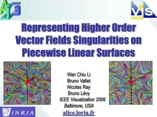
Representing Higher Order Vector Fields Singularities on Piecewise Linear Surfaces. Wan Chiu Li Bruno Vallet Nicolas Ray Bruno Lévy IEEE Visualization 2006 Baltimore, USA alice.loria.fr. Outline. Introduction Discrete representation Singularities Encoding an existing vector field

E N D
Representing Higher Order Vector Fields Singularities on Piecewise Linear Surfaces Wan Chiu Li Bruno Vallet Nicolas Ray Bruno Lévy IEEE Visualization 2006 Baltimore, USA alice.loria.fr
Outline • Introduction • Discrete representation • Singularities • Encoding an existing vector field • LIC-based visualization • Conclusion
Introduction • What is a vector field singularity ? • It is a 0 of the field • How can we characterize singularities ? • By their index = ∫ dθ -1 +1
Introduction • What is a vector field singularity ? • It is a 0 of the field • How can we characterize singularities ? • By their index = ∫ dθ -2 +2
Introduction • How can we visualize a singularity ? • Piecewise linear methods: index∊[-val/2+1, val/2+1] [Tricoche00]
Introduction • How can we visualize a singularity ? • Piecewise linear methods: index∊[-val/2+1, val/2+1] • Higher order singularities: index∊ℤ
Introduction • Basic idea: • 2D vectors are complex reiθ • Interpolate r and θ • Justification: • Singularity = (r =0, θ undefined) • Singularity index depend only on θ in neighborhood
Discrete representation • On triangulated meshes • Dual vertex-edge encoding using polar coordinates: • Dual vertices: norm r∊ℝ, angle θ∊ℝ • Dual edges: period jump p∊ ℤ • 3 Step interpolation (0D, 1D, 2D) • Dual vertices=Facet centers (0D) • Dual edges (1D) • Subdivision simplex (2D)
0D r(v*) θ(v*) v* x(v*) • θ(v*) : measured from a reference vectorx(v*) • r(v*) : vector norm, basis independent
1D v* θ(v*) P v’* x(v*) e* θ(v’*) x(v’*) Linear interpolation: θ(P) = θ(v*) + ∆θ(e*)⍺(e*)t ⍺(e*): height ratio, ∆θ(e*): angular variation alonge*
1D v* θ(v*) v’* P x(v*) e* θ(v’*) x(v’*) Linear interpolation: θ(P) = θ(v*) + ∆θ(e*)(1-⍺(e*))t ⍺(e*): height ratio, ∆θ(e*): angular variation alonge*
1D v* Height ratio: ⍺(e*) =h/H 1-⍺(e*) =h’/H e* h H h’ v’*
1D Angular variation alonge* : Period Jump: ∆θ(e*)= ∫dθ = θ(B) -θ(A) + 2 πp(e*) e* B p(e*) = -1 e* A B p(e*) = 0 e* A B p(e*) = 1 e* A
2D Subdivision simplex
2D Subdivision simplex
2D • A variant the side-vertex interpolation [Nielson79] • Linear along the side • Constant along a side-vertex path (=side value) side P’ P vertex
Singularities • Singularities may occur only at vertices • Singularity indexdepends only on period jumps : • I(v)= ∫dθ = I0(v)+ ∑ p(e*) e*∊∂f* ∂f* f* v
Singularities • Advantages: • Control over placement and index of singularities • Coherent with Poincare-Hopf index theorem • Index independent of the valence • Easy extension to fractional indices
Extension to fractional indices • Fractional indices appear in N-symmetry vector fields : • Not vectors but equivalence class of vectors by ≡N • u≡Nv ⇔ ∃k | u=R(v, 2kπ/N) • Period jump and Indices are multiples of 1/N -1/2 +1/2
Extension to fractional indices • Fractional indices appear in N-symmetry vector fields : • Not vectors but equivalence class of vectors by ≡N • u≡Nv ⇔ ∃k | u=R(v, 2kπ/N) • Period jump and Indices are multiples of 1/N -1/4 +1/4
Encoding an Existing Vector Field • r(v*) : norm of the vector at facet center v* • θ(v*): choose one of the 3 edges and compute angle • 2πp(e*)=∆θ(e*) - ∠(x(v’*), x(v*)) - θ(v’*) + θ(v*) • Requires an interpolation or an analytic form: vxdvy – vydvx ∆θ= ∫dθ = ∫ ||v||2 e* e*
Encoding an Existing Vector Field ∆θ= ∫dθ = ∫ (vxdvy – vydvx) / ||v||2 e* e* dθ v* v’* e*
LIC-based Visualization • GPU accelerated • Works in image space • 3 passes [Laramee et. al. 03] [Van Wijk 03] Ensure geometric discontinuity (in depth buffer) Line integral convolution (in image space) Direction on the surface (in fragment shader)
Results Index = -3 Index = 5
Conclusion • Dual vertex-edge encoding • + 3 steps interpolation: • A very good candidate for visualizing non-linear vector fields on piecewise linear surfaces or 2d meshes. • Efficient and simple way to visualize arbitrary singularities • Easy generalization to fractional indices • Easier particularization to 2d fields
Future work • Smooth non singular vertices • Topological operations • Trace streamlines • Extension to 3d vector fields
alice.loria.fr Questions ?