Coping with Variability in Dynamic Routing Problems
180 likes | 298 Vues
This paper explores dynamic routing problems characterized by inherent variability in travel times. Traditional deterministic models overlook this variability, leading to less effective routing solutions. We propose a queueing framework to analyze travel time distributions, modeling them with lognormal distributions to improve optimization. We employ advanced heuristics like Ant Colony Optimization and Tabu Search and observe significant gains of over 15% in travel times. Our findings indicate that embracing travel time variability can lead to more robust solutions, minimizing re-planning needs and enhancing routing efficiency.

Coping with Variability in Dynamic Routing Problems
E N D
Presentation Transcript
Coping with Variability in Dynamic Routing Problems Tom Van Woensel (TU/e) Christophe Lecluyse (UA), Herbert Peremans (UA), Laoucine Kerbache (HEC) and Nico Vandaele (UA)
Previous work • Deterministic Dynamic Routing Problems • Inherent stochastic nature of the routing problem due to travel times • Average travel times modeled using queueing models • Heuristics used: • Ant Colony Optimization • Tabu Search • Significant gains in travel time observed • Did not include variability of the travel times
Speed vf Speed-density diagram Speed-flow diagram v2 v1 Density Traffic flow k1 kj k2 q qmax q qmax Flow-density diagram Traffic flow A refresher on the queueing approach to traffic flows
Queue Service Station (1/kj) Queueing framework Queueing T: Congestion parameter
Travel Time Distribution: Mean • P periods of equal length Δp with a different travel speed associated with each time period p (1 < p < P) • TT k * p • Decision variable is number of time zones k • Depends upon the speeds in each time zone and the distance to be crossed
Travel Time Distribution: Variance I • TT k * p (Previous slide) Var(TT) p2 Var(k) • Variance of TT is dependent on the variance of k, which depends on changes in speeds • i.e. Var(k) is a function of Var(v) • Relationship between (changes in k) as a result of (changes in v) needs to be determined: k = v
Speed v A vavg v B t0 Time zones k Travel Time Distribution: Variance III Area A + Area B = 0k = v
Travel Time Distribution: Variance IV • k v (and ~ f(v, kavg, p)) Var(k) 2 Var(v) • Var(v) ?
Travel Time Distribution: Variance V • What is Var(1/W)? • Not a physical meaning in queueing theory • Distribution is unknown but: • Assume that W follows a lognormal distribution (with parameters and ) • Then it can be proven that: (1/W) also follows a lognormal distribution with (parameters - and ) • See Papoulis (1991), Probability, Random Variables and Stochastic Processes, McGraw-Hill for general results.
Travel Time Distribution: Variance VI With (1/W) following a Lognormal distribution, the moments of its distribution can be related to the moments of the distribution for W as follows: W ~ LN
Travel Time Distribution • If W ~ LN 1/W ~ LN v~ LN TT~ LN • Assumption is acceptable: • Production management often W ~ LN • E.g. Vandaele (1996); Simulation + Empirics • Traffic Theory often TT ~ LN • Empirical research: e.g. Taniguchi et al. (2001) in City Logistics
Travel Time Distribution: Overview • TT ~ Lognormal distribution E(W) and Var(W) see e.g. approximations Whitt for GI/G/K queues
Finding solutions for the Stochastic Dynamic Routing Problem Data generation: Routing problem Traffic generation Heuristics Ant Colony Optimization Tabu Search Solutions
Objective Functions I • Results for F1(S): • Significant and consistent improvements in travel times observed (>15% gains) • Different routes
Objective Functions II • Objective Function F2(S) • No complete results available yet • Preliminary insights: • Not necessarily minimal in Total Travel Time • Variability in Travel Times is reduced • Recourse: Less re-planning is needed • Robust solutions
Conclusions • Travel Time Variability in Routing Problems • Travel Times • Lognormal distribution • Expected Travel Times and Variance of the Travel Times via a Queueing approach • Stochastic Routing Problems • Time Windows !