The LHCb Computing TDR
The LHCb Computing TDR. Domenico Galli, Bologna. INFN CSN1 Napoli, 22.9.2005. Outline. LHCb software; Distributed Computing; Computing Model; LHCb & LCG; Milestones; LHCb request for 2006. LHCb Software Framework.

The LHCb Computing TDR
E N D
Presentation Transcript
The LHCb Computing TDR Domenico Galli, Bologna INFN CSN1 Napoli, 22.9.2005
Outline • LHCb software; • Distributed Computing; • Computing Model; • LHCb & LCG; • Milestones; • LHCb request for 2006. The LHCb Computing TDR. 2 Domenico Galli
LHCb Software Framework • LHCb software has been developed inside a general Object Oriented framework (Gaudi) designed to provide a common infrastructure and environment for the different software applications of the experiment. • Use of the framework discipline in all applications helps to ensure the integrity of the overall software design and results in maximum reuse of the core software components. • Gaudi is architecture-centric, requirements-driven framework: • Adopted by ATLAS; used by GLAST & HARP. • Same framework used both online & offline. The LHCb Computing TDR. 3 Domenico Galli
Object Diagram of the Software Framework The LHCb Computing TDR. 4 Domenico Galli
Gaudi Design Choices • Decoupling between the objects describing the data and the algorithms. • Distinguish between a transient and a persistentrepresentation of the data objects. • Data flow between algorithms proceeds via the so-called Transient Store. • Same classes for real and MC data. Clear separation between reconstructed data and the corresponding Monte Carlo Truth data (connection through smart references). • Interfaces (pure abstract classes in C++) developed independent of their actual implementation. • Run-time loading of components (dynamic libraries). The LHCb Computing TDR. 5 Domenico Galli
DataObject AlgorithmObject NewDataObject Decoupling between Data and Algorithms • OO modeling should mimics the real world. • The tasks of event simulation, reconstruction and analysis consist of the manipulation by algorithms of mathematical or physical quantities such as points, vectors, matrices, hits, momenta etc. • This kind of task maps naturally onto a procedural language such as Fortran, which makes a clear distinction between data and code. • A priori, there is no reason why using an object-oriented language such as C++ should change the way of doing physics analysis. • Allows programmers to concentrate separately on both data and algorithms. • Allows a longer stability for the data objects as algorithms evolve much more rapidly. • Data objects (the LHCb Event Model) • Provide manipulation of internal data members: onlycontain enough basic internal functionality for givingalgorithms access to their content and derived information. • Algorithms and tools: • Perform the actual data transformations: process data objects of some type and produce new data objects of a different type. The LHCb Computing TDR. 6 Domenico Galli
Transient and Persistent Data • Gaudi make a clear distinction between a transient and a persistent representation of the data objects, for all categories of data. • Algorithms see only data objects in the transient representation: • Algorithms are shielded from the technology chosen to store the persistent data objects. • We have changed from ZEBRA to ROOT/IO to LCG POOL without the physics code encapsulated in the algorithms being affected. • The two representations can be optimized following different criteria (e.g. execution vs. I/O performance). • Different technologies can be accessed (e.g. for thedifferent data types). The LHCb Computing TDR. 7 Domenico Galli
DataObject AlgorithmObject NewDataObject The Data Flow between the Algorithms • The Data Flow between the Algorithms proceeds via the Transient Event Store. • Algorithms retrieve their input data on the TES, and publish their output data to the TES. • 3 categories of data with different lifetime: • Event data (valid for the time it takes to process one event). • Detector data (valid as long as detector conditions don’t change). • Statistical data (lifetime corresponding to a complete job). • Transient store is organized in a tree-like structure. • Data item logically related grouped in containers. • Algorithms may not modify data already on the TES, and may not add new objects to existing containers. • A given container can only be manipulated by the algorithm that publishes it on the TES. • Ensures that subsequent algorithms that are interested in this data can be executed in any order. The LHCb Computing TDR. 8 Domenico Galli
Smart References • Clear separation between reconstructeddata and corresponding Monte CarloTruth data. • No references in Digits that allowtransparent navigation to thecorresponding MC Digits. • This allows using exactly the same classesfor reconstructed real data andreconstructed simulated data. • The relationship to Monte Carlo ispreserved by the fact that the MC Digits and the Digits use the unique electronics channel identifier as a Key. • Smart references implements the relationships between objects in different containers. • From the class further in the processing sequence towards the class earlier in the sequence. • Linkers and Relations implements relationship between object distant in the processing chain. The LHCb Computing TDR. 9 Domenico Galli
LHCb Data Processing Applications and Data Flow The LHCb Computing TDR. 10 Domenico Galli
LHCb Data Processing Applications and Data Flow (II) • Each application is a producer and/or consumer of data for the other applications. • The applications are all based on the Gaudi framework: • Communicate via the LHCb Event model and make use of the LHCb unique Detector Description. • Ensures consistency between the applications and allows algorithms to migrate from one application to another as necessary. • Subdivision between the different applications has been driven by: • Different scopes (simulation and reconstruction); • Convenience (simulation and digitization); • CPU consumption and repetitiveness of the tasks performed (reconstruction and analysis). The LHCb Computing TDR. 11 Domenico Galli
Event Sizes & Processing Requirements The LHCb Computing TDR. 12 Domenico Galli
Version Production version: VELO: v3 for T<t3, v2 for t3<T<t5, v3 for t5<T<t9, v1 for T>t9 HCAL: v1 for T<t2, v2 for t2<T<t8, v1 for T>t8 RICH: v1 everywhere ECAL: v1 everywhere Time VELO alignment HCAL calibration RICH pressure ECAL temperature t1 t2 t3 t4 t5 t6 t7 t8 t9 t10 t11 Time = T Data source Conditions DB • Tools and framework to deal with conditions DB and non-perfect detector geometry is in place. • LCG COOL project is providing the underlying infrastructure for conditions DB. The LHCb Computing TDR. 13 Domenico Galli
Distributed Computing • LCG (LHC Computing Grid): • Set of baseline services for Workload Management (job submission and follow-up) and Data Management (storage, file transfer, etc.). • DIRAC (Workload Management tool)& GANGA (Distributed Analysis Tool): • Higher level services which are experiment dependent. • DIRAC has been conceived as a lightweight system with the following requirements: • be able to accommodate evolving grid opportunities; • be easy to deploy on various platforms: • other resources provided by sites not participating to the LCG; • a large number of desktop workstations; • Present all the heterogeneous resources as single pool to a user. • Single central Task Queue is foreseen both for production and user analysis jobs. The LHCb Computing TDR. 14 Domenico Galli
DIRAC Architecture Services: provide access to the various functionalities of the DIRAC system in a well controlled way. Agents: lightweight software components running close to the computing and storage resources. Allow the services to carry out their tasks in a distributed computing environment. Resources: represents Grid Computing and Storage elements. Provide access to their capacity and status information. The LHCb Computing TDR. 15 Domenico Galli
DIRAC Interface to LCG • There are several ways to interface DIRAC to LCG: • Sending jobs directly to the LCG Computing Element; • Used in DC 03; • Interfacing DIRAC to the LCG Resource Broker; • Not yet reliable enough in DC 04; • Using Pilot Agents; • Successfully experienced in DC 04. The LHCb Computing TDR. 16 Domenico Galli
DIRAC Pilot Agent • The jobs that are sent to the LCG-2 Resource Broker (RB) do not contain any particular LHCb job as payload, but are only executing a simple script, which downloads and installs a standard DIRAC agent. • Since the only environment necessary for the agent to run is the Python interpreter, this is perfectly possible on all the LCG sites. • This pilot-agent is configured to use the hosting Worker Node (WN) as a DIRAC CE. • Once this is done, the WN is reserved for the DIRAC WMS and is effectively turned into a virtual DIRAC production site for the time of reservation. • The pilot agent can verify the resources available on the WN (local disk space, CPU time limit, etc.) and request to the DIRAC Job Management Service only jobs corresponding to these resources. • The reservation jobs are sent whenever there are waiting jobs in the DIRAC Task queue eligible to run on LCG. The LHCb Computing TDR. 17 Domenico Galli
Porting Pilot-Agent Technology to EGEE • Work is going on in INFN-Grid to implement the Pilot-Agent Technology into the EGEE middleware. • To be addressed: • Security issues in agent to Job Management Service communication; • Accounting issues. The LHCb Computing TDR. 18 Domenico Galli
GANGA GUI GUI GUI Collective Collective Collective & & & Histograms Monitoring Results Job Options Algorithms Resource Resource Resource Grid Grid Grid Services Services Services GAUDI Program GAUDI Program GAUDI Program GANGA - User Interface to the Grid • Goal • Simplify the management of analysis for end-user physicists by developing a tool for accessing Grid services with built-in knowledge of how Gaudi works. • Required user functionality • Job preparation and configuration. • Jobsubmission, monitoringand control. • Resource browsing,booking, etc. • Done in collaborationwith ATLAS. • Use Grid middleware services: • Interface to the Grid via Diracand create synergy betweenthe two projects. The LHCb Computing TDR. 19 Domenico Galli
Computing Model The LHCb Computing TDR. 20 Domenico Galli
CERN On-line Farm MC calibration data Selected DST+RAW TAG RAWmc data RAW data • CERN • Tier-1s Physics Analysis reconstruction User DST n-tuple User TAG rDST Local Analysis pre-selectionanalysis • Tier-3s Paper DST+RAW TAG The LHCb Dataflow • Tier-2s • On-line Farm • CERN • Tier-1s • CERN • Tier-1s Chaotic job Scheduled job The LHCb Computing TDR. 21 Domenico Galli
LHCb rDST: a Trick to Save Resources • rDST is an intermediate format (final format is DST). • rDST contains the information needed in the next analysis step. • Missing quantities must be re-calculated at next analysis step: • More CPU resources; • Less Disk resources. • Convenient, since additional CPU resources needed to re-calculate these quantities are cheaper than disk needed to store them. • Quantities to be written on rDST chosen in order to optimize costs. The LHCb Computing TDR. 22 Domenico Galli
HLT 1 a = 107 s over 7-month period rDST25 kB/evt RAW25 kB/evt CERNcomputingcentre 200 Hz 60 MB/s 2x10¹⁰ evt/a 500 TB/a b-exclusive 200 Hz rDST (25 kB/evt) pre-selection analysis 0.2 kSi2k•s/evt 2 streams di-muon 600 Hz 2 kHz RAW (25 kB/evt) D* 300 Hz di-muonrDST+RAW 50 kB/evt b-exclusiveDST+RAW100 kB/evt b-inclusiveDST+RAW100 kB/evt D*rDST+RAW50 kB/evt b-inclusive 900 Hz TAG Streaming The LHCb Computing TDR. 23 Domenico Galli
Computing Model - Resource Summary 1 2.4 GHz PIV = 865 Si2k The LHCb Computing TDR. 24 Domenico Galli
Computing Model - Resource Profiles CERN CPU Tier-1 CPU The LHCb Computing TDR. 25 Domenico Galli
Computing Model - Resource Summary (II) The LHCb Computing TDR. 26 Domenico Galli
LHCb & LCG • DC04 (May-August 2004) • 187 Mevts simulated and reconstructed • 61 TiB of data produced • 43 LCG sites used • 50% using LCG resources (61% efficiency pure LCG, 76% with pilot) • DC04v2 (December 2004) • 100 Mevts simulated and reconstructed • DC04 stripping • Helped in debugging CASTOR-SRM functionality • CASTOR-SRM now functional (at CERN, CNAF, PIC) • RTTC production (May 2005) • 200 Mevts simulated (minimum bias) in 3 weeks (up to 5500 jobs simultaneously). The LHCb Computing TDR. 27 Domenico Galli
LHCb & LCG: Large Scale Production in 2005 on the Grid • The RTTC production lasted just 20 days. • The startup was very fast: • In a few days almost all available sites were in production. • System was able to run with 4000 CPUs over 3 weeks, with a peak of over 5500 CPUs. • 168 M events produced (11 M events as final output after L0 trigger cut). The LHCb Computing TDR. 28 Domenico Galli
RTTC-2005 Production Share 5% produced with plain DIRAC sites 95% produced with LCG sites. The LHCb Computing TDR. 29 Domenico Galli
CNAF Tier-1 Share (May-August): Total CPU Time http://tier1.cnaf.infn.it/monitor/LSF/plots/acct/ The LHCb Computing TDR. 30 Domenico Galli
CPU Exploited by LHCb at the CNAF Tier-1 During the Year 2005 • From CNAF LSF monitor: http://tier1.cnaf.infn.it/monitor/LSF/plots/acct/ • (no data available before May 2005) • May 2005: 222 kSi2k; • Jun 2005: 110 kSi2k; • Jul 2005: 76 kSi2k; • Aug 2005: 310 kSi2k; • Average CPU power exploited by LHCb in 120 days: 180 kSi2k = 150 cpu2005 • 1 cpu2005 (3.2 GHz Xeon) = 1.2 kSi2k The LHCb Computing TDR. 31 Domenico Galli
LHCb & LCG - SC3 & Beyond • Storage Elements for permanent storage should have a common SRM interface; • Supports the LCG requirements for SRM (v2.1). • Evaluating for transfer gLite-FTS in Service Challenge 3 (SC3). • Evaluating LCG File Catalog in SC3; • Previously used AliEn FC and LHCb bookkeeping DB. • Uses its own “metadata” catalogue (LHCb Bookkeeping DB); • Implementation based on ARDA metadata interface being tested. The LHCb Computing TDR. 32 Domenico Galli
LHCb Collaboration with the CNAF Tier-1 • LHCb Italian Computing Group is moving furthermore toward a strict collaboration with the Italian Tier-1: • As the LHCb on-line task (Farm Monitor & Control) terminated the boot-strap phase. • Collaboration items: • Parallel File System for Physics Analysis; • STORM for Parallel File System; • Workload Manager benchmarks. The LHCb Computing TDR. 33 Domenico Galli
LHCb Computing Milestones • Analysis at all Tier-1’s - November 2005 • Start data processing phase of DC’06 - May 2006 • Distribution of RAW data from CERN. • Reconstruction/stripping at Tier-1’s including CERN. • DST distribution to CERN & other Tier-1’s. • Alignment/calibration challenge – October 2006 • Align/calibrate detector. • Distribute DB slice – synchronize remote DB’s. • Reconstruct data. • Production system and software ready for data taking - April 2007 The LHCb Computing TDR. 34 Domenico Galli
LHCb Computing Milestones (II) • LHCb envisages a large scale MC production commencing January 2006 ready for use in DC06 in May. It will be order of 100's Mevents. • Physics request will be planned by the end of October. Mainly for: • Physics studies; • HLT studies. • MC production 2006 is not included in DC’06 (it is no more a real “challenge”). • From now on, practically speaking, an almost continuous MC production is foreseen for LHCb: • This support the request of a chunk of computing resources (mainly CPUs) permanently allocated to LHCb, the LHCb Italian Tier-2. The LHCb Computing TDR. 35 Domenico Galli
LHCb Tier-2 (@CNAF): Additional Size and Cost (linear rump-up 2006 → 2008) 3.2 GHz Xeon = 1.2 kSi2k The LHCb Computing TDR. 36 Domenico Galli
LHCb Tier-2 (@CNAF): Additional Infrastructures 1 kSi2k → 110 W 1 TiB → 70 W The LHCb Computing TDR. 37 Domenico Galli
LHCb Requests for 2006 • 200 k€: Tier-2 resources (140 dual-processor box + 1 TiB Disk). • Since resources are allocated at CNAF, resource management could be flexible: • CPUs can be moved from Tier-1 queues to Tier-2 queues and back with software operations. • But Tier-2 have to be logically separated by Tier-1 (e.g.: different batch queues). The LHCb Computing TDR. 38 Domenico Galli
Summary • LHCb has in place a robust s/w framework. • Grid computing can be successfully exploited for production-like tasks. • Next steps: • Realistic Grid user analyses. • Prepare reconstruction to deal with real data: • particularly calibration, alignment, … • Stress testing of the computing model. • Building the Tier-2. The LHCb Computing TDR. 39 Domenico Galli