Introduction to Broadband Processing with Matlab - Seismic Data Analysis
260 likes | 302 Vues
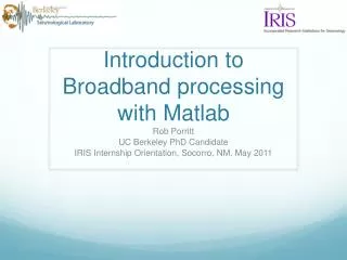
Explore broadband processing techniques in Matlab for seismic data analysis. Learn about preprocessing steps, instrument response removal, integration, and differentiation. Get hands-on experience with provided data and functions.

Introduction to Broadband Processing with Matlab - Seismic Data Analysis
E N D
Presentation Transcript
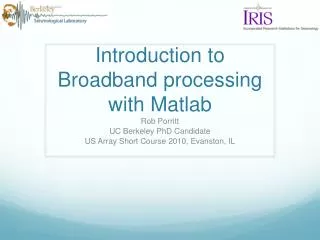
Introduction to Broadband processing with Matlab Rob Porritt UC Berkeley PhD Candidate IRIS Internship Orientation, Socorro, NM. May 2011
Disclaimer • I primarily work in c for the processing speed and my familiarity with it. • The Matlab functions in this tutorial were written by me, a graduate student in seismology, not a computer programmer or an expert in digital signal processing.
Why Matlab? • Pros: • Easy to use and learn • interactive environment • ever-growing library • good documentation • Cons: • Not free • Slow to open • Poor with strings
Matlab packages available • Fissures-MATLAB • Package distributed by IRIS • MatSeis • Package for active source data processing • SplitLab • Package for doing shear-wave splitting
Get your own copy • You can copy the data and functions from my directory on a linux/unix terminal with the command: • cp –r /fs/tmp/porritt_matlab/* . • Now you can call them from matlab or edit them with the editor. • Check out the functions • ls porritt_broadband_processing_matlab/functions
Not just for data processing • Start with a break • Matlab draw poker • poker • Matlab role-playing game • dungeon I made these games years ago during a very boring summer working third shift in an automotive factory.
My favorite equations (1) u(t) = s(t) * g(t) * i(t) or U(ω) = S(ω)G(ω)I(ω) The observed seismogram (u) is a convolution of the source (s) of seismic excitation with the earth’s Green’s function (g) and the convolution with the instrument recording (i). Or in the frequency domain, convolution is multiplication.
My favorite equations (2) ρü = f + (λ + 2μ)∨(∨u) – μ∨ x (∨ x u) The equation of motion in a homogeneous medium, using displacement variables: Or as Sir Isaac Newton put it: MA = ΣF Quantitative Seismology, Aki and Richards, 2002. Equation 4.1
Data • Some data from a Berkeley station is stored in the data/exercise_{1,2,3,5} folders • You can replace that data with your data in the folder data/chile_6.4/ • Inside that folder are three more folders (porritt, miller, anthony) which contain data for a teleseism. • Inside data/ is the pole-zero response of your stations (cmg3t.pz) • Last year’s data is in data/intern_data if you’re interested
Component naming convention • First letter is the sampling rate • L = Low or 1 hz • B = Mid or 40 hz • More options, but these are most likely what you may see • Second letter is the gain • H = High gain • L = Low gain • Third letter is the direction • Z = Vertical • N = North • E = East Thus, BHZ is 40 hz, high gain, vertical
Preprocessing • From here on, the full steps are outlined in the worksheet. • The rest of the presentation will hopefully give background why we do each step, but feel free to start working • Preprocessing is the “standard” steps to get true ground motion from the seismic record • Raw data is in “digital counts” versus time.
Preprocessing • Remove the mean and linear trend • The mean would create a very large DC or 0 frequency amplitude. • The linear trend has a lesser effect, but again amplifies various non-linear effects • Taper the ends • The Discrete Fourier Transform (DFT) algorithm can create significant undesired sidelopes or ringing. Tapering the ends reduces this effect • Remove the instrument response • This is a science in and about itself (see next slide)
Instrument Response • Convolution of sensor, digitizer, and decimation(s). • Sensors has poles to define shape, zeros to define acceleration, velocity, or displacement, and gain for units. • Digitizer does decimation with gain factor and high corner poles • My function does not include digitizer poles and normalization because the sac pole zero file does not contain that information. Amplitude Frequency (Hz)
Integration and Differentiation • We record velocity as a function of time, but moment tensors are defined in terms of displacement and building codes are defined in terms of peak ground accelerations • Thankfully the relations are standard calculus • Sadly they are discrete functions and thus its non-trivial to implement the calculus
Integration and Differentiation • How to integrate or differentiate in the time domain is actually non-trivial. It is thus more common to do frequency domain calculus. • freq_integrate • Divides the data by 2iπf • freq_differentiate • Multiplies the data by 2iπf Displacement Velocity Acceleration
Long period seismograms • Many factors discussed in the worksheet lead to primarily long period signals from large distant earthquake • Large earthquakes excite very large and very long period waves which ring around the earth • The longest period earth mode is the Slichter mode vibrating with a period of around 1 hour.
Exercise • Preprocess the 3-component data to ground velocity • Low pass filter the data • Rotate the horizontals to radial and transverse directions. • If you feel comfortable with Matlab try plotting phases with plot_phases described at the end of the worksheet.
Anthropogenic noise • “Noise” due to human motion typically excites higher frequencies. • High pass filter the data to see the variation between day and night broadband 6am - Berkeley High passed
Power Spectral Density • Spectral estimate of power over a time period • Robust estimates require averaging several spectrums within the time window. • Standard tool for looking at background seismic signals and quality control of stations.
Coherence • Measure of similarity between two signals • Robust estimate via similar method as PSD
Cross Correlation • Estimates delay time of similar signals
Phase arrival estimate Rayleigh? True P? True S? Function still needs work. Main inputs include the distance between station and earthquake, 1D velocity model, depth, and origin time relative to the start of the seismogram.
Generalized Ray Theory • Forward Modeling method. Exercise is not fully developed. Delve into this only if you are exceedingly curious and comfortable with Matlab • Computes the rays with some esoteric law you may have heard of…
Rays computed in code Snell’s Law!