Download
1 / 38
540 likes | 1.37k Vues
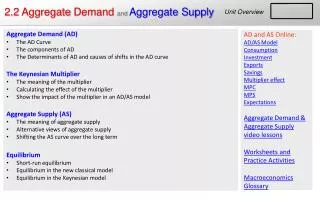
2.2 Aggregate Demand and Aggregate Supply. U nit Overview. Introduction to Aggregate Demand Aggregate Demand: The total demand for the output of a nation at a range of price levels in a particular period of time from all consumers, domestic and foreign.

E N D
2.2 Aggregate Demand andAggregate Supply Unit Overview
Introduction to Aggregate Demand • Aggregate Demand: The total demand for the output of a nation at a range of price levels in a particular period of time from all consumers, domestic and foreign. • Similarities between Aggregate Demand and Demand: • The curve illustrating both slopes downwards, showing an inverse relationship between how much is demanded and prices • There are ‘non-price determinants’ of both demand and aggregate demand. Changes in these factor will cause the curves to shift • A decrease in both causes employment and output to fall. A fall in demand will cause output and employment in a particular industry to decrease; a fall in aggregate demand will cause output and employment in an entire country to decrease. • An increase in both causes prices to rise. A rise in demand will cause the price of a particular good to increase; a rise in aggregate demand causes the average price level in an entire nation to increase (inflation). The Aggregate Demand Curve The Demand Curve Price level Average Price level AD2 D2 D1 AD1 quantity Real Gross Domestic Product (GDP)
Why does the AD Curve Slope Downwards? • The demand for a nation’s output is inversely related to the average price level of the nation’s good. There are three explanations for this: • The wealth effect: Higher price levels reduce the purchasing power or the real value of the nation's households' wealth and savings. The public feels poorer at higher price levels, thus demand a lower quantity of the nation's output when price levels are high. At lower price levels, people feel wealthier and thus demand more of a nation's goods and services. (This is similar to the income effect which explains the downward sloping demand curve).
Why does the AD Curve Slope Downwards? • The demand for a nation’s output is inversely related to the average price level of the nation’s good. There are three explanations for this: • The interest rate effect: In response to a rise in the price level, banks will raise the interest rates on loans to households and firms who wish to consume or invest. At higher interest rates the quantity demanded of products and capital for which households and firms must borrow decreases, as borrowers find higher interest rates less attractive. The opposite results from a fall in the price level and the decline in interest rates, which makes borrowing more attractive and thus increases the quantity of output demanded.
Why does the AD Curve Slope Downwards? • The demand for a nation’s output is inversely related to the average price level of the nation’s good. There are three explanations for this: • The net export effect: As the price level in a particular country falls, ceterus paribus, goods and services produced in that country become more attractive to foreign consumers. Likewise, domestic consumers find imports less attractive as they now appear relatively more expensive, so the net expenditures on exports rises as price level falls. The opposite results from an increase in the price level, which makes domestic output less attractive to foreigners and foreign products more attractive to domestic consumers.
The Components of Aggregate Demand • A change in the average price level of a nation’s output will cause a movement along the AD curve, but a change in other variable will cause the AD curve to shift in or out. The components of aggregate demand are the four types of national expenditures used in GDP • Household Consumption • Capital Investment • Government spending • Net Exports The Aggregate Demand Curve Average Price level P1 AD2 AD1 AD3 Y1 Y2 Y3 Real Gross Domestic Product (rGDP)
The Components of Aggregate Demand – Consumption (C) As one of the components of aggregate demand, consumption refers to all the spending done by households on goods and services. The level of consumption in a nation depends on several factors.
The Components of Aggregate Demand – Investment (I) Investment is the second component of a nation's aggregate demand. Investment is defined as spending by firms on capital equipment or technology and by households on new homes.
The Investment Demand Curve (for loanable funds) The real interest rate is the most important determinant of the level of investment in a nation. Study the graph below to understand the relationship between interest rates and investment. • The Investment Demand Curve: The graph shows the demand for loanable funds, which borrowers need to invest in capital or new homes. Notice: • With a real interest rate of 8%, few firms will want to invest in new capital • When real interest rates are 3%, the quantity of funds demanded for investment is much higher • Firms will only invest if they expect the returns on the investment to be greater than the real interest rate (marginal benefit must be greater than the marginal cost) Investment Demand 8% real interest rate 3% DI Q2 Q1 Quantity of Funds Demanded for Investment
Shifts in the Investment Demand Curve As a component of aggregate demand, the level of investment in the economy depends primarily on the interest rate, but also on other determinants of investment. • If one of the determinants of investment changes, the level of investment will increase or decrease at every interest rate • If business confidence improves, a new technology is developed, business taxes are lowered, firms are producing at full capacity or producers expect higher future prices, • Investment demand will shift from Di to D2 • If business confidence worsens, business taxes increase, firms have lots of excess capacity or producers expect prices to be lower in the future, Investment demand will shift from Di to D3. Investment Demand real interest rate 5% D2 D3 DI Q2 Q1 Q3 Quantity of Funds Demanded for Investment
The Components of Aggregate Demand – Net Exports (Xn or X-M) Another components of the total demand for a nation’s output is export revenues. Net exports refers to the revenue earned from the sale of exports to the rest of the world minus the expenditures made on imports from abroad. Net exports equals exports (X) – imports (M)
The Components of Aggregate Demand – Government Spending (G) • Government spending is the final component of aggregate demand. The level of government spending in a nation is determined by the government’s fiscal policy. • Fiscal Policy: Changes in the levels of taxation and government spending meant to expand or contract the level of aggregate demand in a nation to promote macroeconomic objectives such as full employment, stable price and economic growth. There are several key concepts relating to fiscal policy to consider: • Contractionary fiscal policy: If the government reduces its spending and / or increases the level of taxation, aggregate demand will decrease and shift to the left • Expansionary fiscal policy: If the government increases its expenditures and / or decreases the level of taxation, aggregate demand will increase and shift to the right. • Budget deficit: If, in a particular year, a government runs a deficit, meaning its expenditures exceed tax revenues, then government spending will contribute to AD that year and cause it to increase and shift out. • Budget surplus: If, in a particular year, a government runs a surplus, meaning it spends less than it collected in taxes, then fiscal policy will subtract from aggregate demand, shifting it to the left.
Shifts of the AD 2.2 Wrksht Price Level D2 D3 DI Q2 Q1 Q3 OUTPUT
Fiscal Policy’s Affect on Aggregate Demand In 2007 the US was about to enter a recession. In response, the government announced an expansionary fiscal policy aimed at increasing AD. The table below summarizes the components of and the desired effects of the government’s policy.
The Marginal Propensities As national income rises or falls, the level of consumption among households varies based on the marginal propensity to consume. Besides consuming with their incomes, households also save, pay taxes and buy imports. The proportion of any change in income that goes towards each of these is known as the marginal propensity • The Marginal Propensity to Consume (MPC): this is the proportion of any change in national income (Y) that goes towards consumption (C) by households: • The Marginal Propensity to Save (MPS): The proportion of any change in national income (Y) that goes towards savings (S) by households: • The Marginal Propensity to Import (MPM): The proportion of any change in national income (Y) that goes towards buying imports (M) by households: • The Marginal Rate of Taxation (MRT): The proportion of any change in national income (Y) that goes towards paying taxes (T) by households: Consumption is a component of AD, while savings, buying imports, and paying taxes are all leakages from the nation’s circular flow. These three together are known as the marginal rate of leakage (MRL). These are the four things households can do with any change in their income. Therefore,
Calculating Marginal Propensities to Consume and Save Study the table below, which shows how consumption, taxes, savings and imports change following a $1 trillion increase in US households income. 2 2 2
Calculating Marginal Propensities to Consume and Save Study the table below, then answer the questions that follow: Source: http://www.bea.gov/ Describe the changes in US personal income between each of the years from 1999-2007. Calculate the marginal rate of taxation for each of the years () Calculate the marginal propensity to save for each of the years () Calculate the marginal propensity to consume for each of the years (in this table, consumption is referred to as ‘personal outlays’. () Personal consumption ("personal outlays") and Personal savings in the US MPC
The Spending Multiplier and Aggregate Demand • When a particular component of AD changes (either C, I, Xn or G) the change in total spending the economy experiences will be greater than the initial change in expenditures. This is known as the multiplier effect. • Example of the multiplier effect in action: Assume the US government decides to increase spending on infrastructure project (roads, bridges, etc…) by $100 billion. What happens to this money? • $100 billion will be earned by households employed in the infrastructure projects. • Of that, some percentage will be saved, paid in taxes and used to buy imports. But some percentage will be used for consumption. • The income earned from the $100 billion government spending and then spent on consumption be earned again by other households! • Assume that the MPC = 0.8. this means that of the $100 billion, $80 billion will be spent again by the households that earned it. There is now an additional $80 billion of new income, of which… • $64 billion will be spent again (0.8 x 80). In this way, the initial change in government spending of $100 billion is MULTIPLIED throughout the economy to create even more total spending. • The size of the Multiplier is determined by the MPC, and can be calculated as:
The Spending Multiplier and Aggregate Demand The table below shows the changes in total spending that will result from an initial change in expenditures of $100 in an economy, based on different marginal propensities to consume. Study the data and then answer the questions that follow. What is the relationship between the MPC and the size of the spending multiplier? What is a logical explanation for this relationship? Under what circumstance will a particular increase in government spending be most effective, when the MPC is low or when it is high? Does the multiplier effect work when the initial change in spending is negative? What would this mean for an economy in which business confidence is falling?
The Spending Multiplier and Aggregate Demand The effects of the spending multiplier can be seen on an aggregate demand curve. Assume, for example, an economy experiences $50 million increase in its net exports (perhaps due to a depreciation of its currency). The MPC in this economy is 0.6. The Aggregate Demand Curve • The Spending Multiplier = • Initial change in spending = $50 million • The effect of the initial increase in Xn is shown by a shift from AD1 to AD2. At P1, the level of output demanded only increases to Y2 • Final change in spending = $50 million x 2.5 = $125 million • The ultimate effect on AD will be a shift to AD3. Assuming the price level remained at P1, the total demand for output is now at Y3. Average Price level P1 AD3 AD2 AD1 Y1 Y2 Y3 Real Gross Domestic Product (rGDP)
The Tax Multiplier and Aggregate Demand When a component of AD changes, total spending will change depending on the spending multiplier. But a factor that determines one of the components of AD changes (taxes in this case), the effect on AD will be less direct. The Tax Multiplier: When the government reduces taxes by a certain amount, households’ disposable income increases, and therefore consumption increase, leading to an increase in AD. The tax multiplier tells us the amount by which total spending will increase following an initial decrease in taxes of a particular amount. Remember, the MRL is the marginal rate of leakage. It refers to the things households do with any change in incomethat do not contribute to the nation’s total demand*. Why two formulas? Two formulas are provided because in AP Economics, students are not expected to learn the MRL. The assumption is that MPC+MPS=1. However, in IB Economics, we must consider the MPS, MPM and the MRT, so MPC+MRL=1. The formulas are the same, but while IB students must remember the one on the left, AP student need only consider the one on the right.
The Tax Multiplier and Aggregate Demand If we know the MPC for a country, and we know how much taxes are cut by, we can calculate the tax multiplier and determine the ultimate change in total spending that will result from the tax cut. Remember that the MRL is always equal to 1-MPC. Notice that at every level of MPC, the change in total spending that results from a $100 tax cut is LESS THAN the change in total spending that resulted from a $100 increase in spending (from an earlier slide). The tax multiplier will ALWAYS be smaller than the spending multiplier, a proportion of any tax cut will be leaked before it is spent.
The Determinants of Aggregate Supply • The Determinants of Aggregate Supply: When any of the following change, aggregate supply will either decrease and shift inwards (or up, graphically) or increase and shift outwards (or down, graphically). • Wage rates:. Higher wages cause SRAS to decrease, lower wages cause SRAS to increase • Resource costs: Rents for land, interest on capital; as these rise and fall, so does AS • Energy and transportation costs: Higher oil or energy prices will cause SRAS to decrease. If costs fall, SRAS increases • Government regulation: Regulations impose costs on firms that can cause SRAS to decrease • Business taxes: Taxes are a monetary cost imposed on firms by the government, and higher taxes will cause SRAS to decrease • Exchange rates: If a country’s producers use lots of imported raw materials, then a weaker currency will cause these to become more expensive, reducing SRAS. A stronger currency can make raw materials cheaper and increase AS.
Background on the Competing Views of Aggregate Supply The vertical, long-run aggregate supply curve reflects the theories of a school of economic thought known as the new (or neo)-classical school of economics. What follows is a brief background of the new-classical theory of aggregate supply. The Classical view of Aggregate Supply: During the boom era of the Industrial Revolutions in Europe, Britain and the United States, governments played a relatively small role in nation’s economies. Economic growth was fueled by private investment and consumption, which were left largely unregulated and unchecked by government. When labor unions were weak and minimum wages and unemployment benefits were unheard of, wages fluctuated depending on market demand for labor. When spending in the economy was strong, wages were driven up and firms restricted their output in response to higher costs, keeping output near the full employment level. When spending in the economy was weak, firms lowered workers' wages without fear of repercussions from unions or government requiring minimum wages. Flexible wages meant labor markets were responsive to changing macroeconomic conditions, and economies tended to correct themselves in times of excessively weak or strong aggregate demand. The Classical view of aggregate supply held that left unregulated, a weak or over-heating economy would "self-correct" and return to the full-employment level of output due to the flexibility of wages and prices. When demand was weak, wages and prices would adjust downwards, allowing firms to maintain their output. When demand was strong, wages and prices would adjust upwards, and output would be maintained at the full-employment level as firms cut back in response to higher costs. In the new-classical view, the aggregate supply curve is always VERTICAL
Background on the Competing Views of Aggregate Supply The upwards sloping, short-run aggregate supply curve reflects the theories of a school of economic thought known as the Keynesian school. What follows is a brief background to the Keynesian view of AS. The Keynesian View of Aggregate Supply: John Maynard Keynes was an English economist who represented the British at the Versailles treaty talks at the end of WWI. During the Great Depression, Keynes noticed that, in contrast to what the neo-classical economists thought should happen, the world’s economies were not self-correcting. Keynes believed that during a time of weak spending (AD), an economy would be unable to return to the full-employment level of output on its own due to the downwardly inflexible nature of wages and prices. Since workers would be unwilling to accept lower nominal wages, and because of the role unions and the government played in protecting worker rights, the only thing firms could due when demand was weak was decrease output and lay off workers. As a result, a fall in aggregate demand below the full-employment level results in high unemployment and a large fall in output. To avoid deep recession and rising unemployment after a fall in private spending (C, I, Xn), a government must fill the "recessionary gap" by increasing government spending. The economy will NOT "self-correct" due to "sticky wages and prices", meaning there should be an active role for government in maintaining full-employment output. In the Keynesian view, AS is horizontal below full-employment and vertical beyond full employment!
Background on the Competing Views of Aggregate Supply The extreme Keynesian view of is seen as a horizontal curve and the extreme new-classical view of AS is seen as a vertical curve. The Classical view The Keynesian view PL PL AS AS Yfe Yfe real GDP real GDP
Background on the Competing Views of Aggregate Supply • In reality, neither view is totally correct. • Keynes was right in the short-run, because wages and prices tend not to adjust quickly to changes in the level of demand. • The new-classicists are right in the long-run, because over time, The Classical view The Keynesian view PL PL AS AS following a decrease or an increase in AD, wages and prices tend to rise or fall accordingly, causing output in the nation to return to a relatively constant, full-employment level, regardless of the level of AD. Yfe Yfe real GDP real GDP
Short-run Aggregate Supply The Keynesian theory of relatively inflexible wages and prices is reflected in the short-run aggregate supply curve, which is relatively flat below full employment (Yfe) and relatively steep beyond full employment. SRAS PL P4 Pfe P3 P2 P1 Y2 Y3 Yfe Y1 Y4 real GDP
Long-run Aggregate Supply The new-classical view of AS is reflected in the vertical, long-run AS curve, which shows that output will always occur at the full employment level (Yfe). LRAS SRAS PL P4 Pfe P3 P2 P1 Y2 Y3 Yfe Y1 Y4 real GDP
Short-run Equilibrium in the AD/AS Model – Full Employment By considering both the aggregate supply AND the aggregate demand in a nation, we can analyze the levels of output, employment and prices in an economy at any particular period of time. Consider the economy shown here: LRAS SRAS • When equilibrium occurs at full-employment: • The total demand for the nation’s output is just high enough for the economy to produce at its full employment level in the short-run. • Nearly everyone who wants a job has a job and the nation’s capital and land are being fully utilized. Unemployment is at its Natural Rate (the NRU) • Since the economy is at full-employment, we can assume that the macroeconomic objectives are being met: • Price level stability, • Full employment • Economic growth. PL Pfe AD1 Yfe real GDP
Short-run Equilibrium in the AD/AS Model – AD decreases On the previous slide the economy was producing at full employment level, e.g. a strong, healthy economy. But what if AD fell due to a fall in consumption, net exports, investment or government spending? LRAS SRAS PL • At AD2: • A fall in expenditures has caused AD to decrease to AD2 • In the short-run, firms will fire workers and reduce output to Y2. Price level fall, but only slightly, to P2 • The economy is no longer at full employment, and is in a demand-deficient recessionat Y2. • Price level has fallen slightly • Employment has decreased • National output has decreased, there is a recessionary gap equal to the difference between actual output and full-employment output Pfe P2 AD1 AD2 Y2 Yfe real GDP Recessionary Gap
Long-run Equilibrium in the AD/AS Model: AD decreases • At AD2 in the long-run: • Over time, unemployed workers will begin accepting lower wages, which will reduce production costs for firms • At lower wage rates, SRAS increases to SRAS1, firms begin hiring back the workers they fired when AD first fell • Output will return to Yfe, and prices will fall to Pfe1. The economy “self-corrects” in the long-run • Output returns to full employment • Wages are lower, but prices are too • The economy recovers on its own from the recession in the long-run LRAS SRAS PL SRAS1 P2 AD1 Pfe1 AD2 Y2 Yfe real GDP
Short-run Equilibrium in the AD/AS Model – AD increases Next let’s examine what happens in the short-run when AD increases. Assume below that either consumption, investment, net exports or government spending increased, causing the AD curve to shift from AD1 to AD3 • At AD3: • An increase in demand led to firms wanting to produce more output, which increases to Y3. • Wages are relatively inflexible in the short-run, so firms can hire more workers, and the economy produces beyond its full employment level. • The economy experiences demand-pull inflation • Price level has risen due to greater demand for the nation’s output • Employment has increased • The economy is beginning to ‘overheat’, and there is an inflationary gapequal to the difference between actual output and full-employment output LRAS SRAS PL P3 AD3 Pfe AD1 Inflationary Gap Yfe Y3 real GDP
Long-run Equilibrium in the AD/AS Model – AD increases In the long-run, wages and prices will adjust to the level of aggregate demand in the economy. When AD grows beyond the full employment level, this means wages will rise in the long-run, leading producers to reduce employment and output back to the full-employment level LRAS • At AD3 in the long-run: • Demand for resources has driven up their costs (wages, rents, interest have all risen) • Facing rising costs of production, firms begin reducing employment and output, and passing higher costs onto consumers as higher prices. • Output returns to Yfe, and price level rises to Pfe3 • The economy has self-corrected from the rising AD • Output is back at its full-employment level • There is more inflation in the economy (higher price levels) SRAS1 PL SRAS Pfe3 P3 AD2 AD1 Yfe real GDP
Negative Supply Shocks - Stagflation Assume that a determinant of AS changes which causes the short-run aggregate supply curve to decrease, and shift to the left. What results is a situation known as stagflation LRAS • Stagflation: An increase in the average price level combined with a decrease in output, caused by a negative supply shock. “Stagnant growth” and “inflation” together make “stagflation” • Assume higher energy costs caused SRAS to decrease to SRAS2. • To off-set higher energy costs, firms must lay off workers, reducing employment. • Higher costs must be passed onto consumer as higher prices, causing inflation. • An economy facing stagflation will only self-correct if resources costs fall in the long-run, which may occur if wages fall due to a large increase in unemployment. SRAS2 PL SRAS1 P2 Pfe AD Y2 Yfe real GDP
Positive Supply Shocks – Economic Growth While a negative supply shock can be disastrous for an economy, a positive supply shock has very beneficial effects on employment, output and the price level. Assume ,for example, a nation signs a free trade agreement and now lots of new resources can be imported at very low costs. LRAS PL • SRAS increases to SRAS3: • Cheaper resource costs allow firms to produce more output with the same amount of workers and capital. • Lower costs are passed onto consumers as lower prices, Pfe falls to P3 • Output increases to Y3, indicating short-run economic growth has occurred. • If the lower costs remain permanent, then eventually LRAS will increase and Y3 will become the new full-employment level of output, indicating long-run economic growth SRAS1 SRAS3 Pfe P3 AD Y3 Yfe real GDP
Long-run Economic Growth in the AD/AS Model So far we have illustrated demand-deficient recessions, demand-pull inflation, negative and positive supply shocks. But real, long-run economic growth requires that not only AS or AD increase, rather that both AS AND AD increase. LRAS1 LRAS2 • Long-run Economic Growth: • For national output to grow in the long-run, AD, SRAS and LRAS must all shift outward. • This can be cause by an improvement in the production possibilities of the nation, combined with growing demand for the nation’s output. • The quality and/or quantity of resources must increase: • Better technology, • Larger population, • Better educated workforce, • More natural resources, and so on. PL SRAS1 SRAS2 Pfe AD1 AD2 Yfe2 Yfe1 real GDP
2.2 Aggregate Demand andAggregate Supply Equilibrium Video Lesson AN INTRODUCTION TO AGGREGATE SUPPLY – FROM SHORT-RUN TO LONG-RUN