Sensor Networks

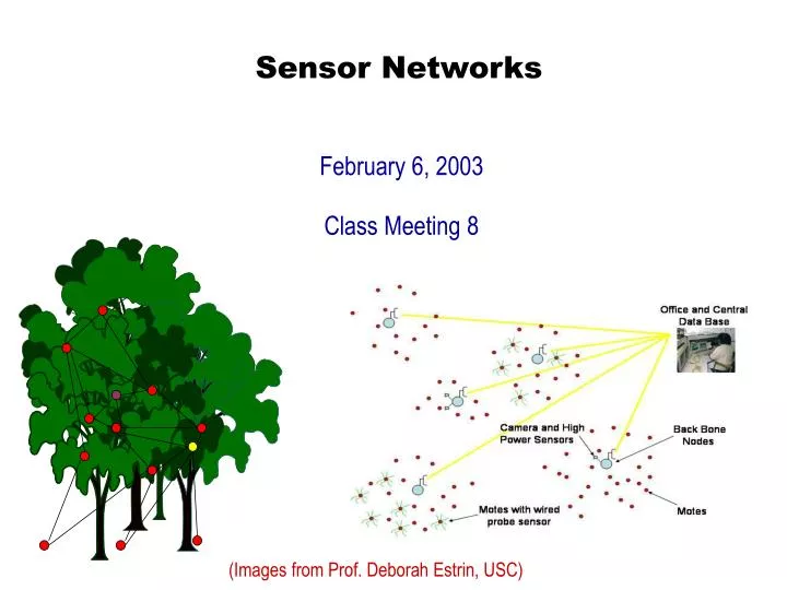
1. Sensor Networks February 6, 2003 Class Meeting 8 (Images from Prof. Deborah Estrin, USC)

2. Objectives • Embedded Sensor Networks • How to coordinate distributed sensor nodes?

3. Once We Have a Blanket/Field CoverageHow Do We Handle Sensor Data? • Lots of sensors distributed over wide area, each with only local information

4. Example: Intruder Detection UsingDistributed Acoustic Sensor Network Distributed Acoustic Sensing Algorithm: While (forever) • Communicate my volume heard (h) to my nearest neighbors; • Receive V[1..n] volumes from my n nearest neighbors; • If h > V[i], for all i, then: • Broadcast my position as nearest to the detected target

5. Embedded Networked Sensing (ENS):A Transforming Technology • Imagine if: • High-rise buildings in Los Angeles were able to detect their own structural faults (e.g., weld cracks or plumbing infrastructure) • Buoys along the coast could alert surfers, swimmers, and fisherman to dangerous bacterial levels • An earthquake-rubbled building could be infiltrated with robots and sensors to locate signs of life and evaluate structural damage • We could infuse complex and endangered ecosystems with a plethora of chemical, physical, acoustic, and image sensors to track global change parameters continuously. • Dangerous bacterial and contaminant levels could be detected “on the farm” through dense sampling, instead of “in the market” through sparse sampling (Slide adapted from Prof. Deborah Estrin, USC)

6. Embedded Networked Sensing Potential • Micro-sensors, on-board processing, and wireless interfaces all feasible at very small scale: • Can monitor phenomena “up close” • Enables spatially and temporally dense environmental monitoring • Revealspreviously unobservable phenomena Seismic Structure Response Contaminant Transport Ecosystems, Biocomplexity Marine Microorganisms (Slide adapted from Prof. Deborah Estrin, USC)

7. Disaster Response Circulatory Net More Examples… Embednumerous distributed devices to monitor and interact with physical world: work-spaces, hospitals, homes, vehicles, and “the environment” Network these devices so that they can coordinate to perform higher-level tasks. Requires robust distributed systemsof hundreds or thousands of devices. (Slide adapted from Prof. Deborah Estrin, USC)

8. Enabling Technologies Embednumerous distributed devices to monitor and interact with physical world Network devices tocoordinate and perform higher-level tasks Embedded Networked Exploit collaborative sensing, action Control system with small form factor, untethered nodes Sensing Tightly coupled to physical world Exploit spatially and temporally dense, in situ, sensing and actuation (Slide adapted from Prof. Deborah Estrin, USC)

9. “The network is the sensor” (Manges & Smith, Oak Ridge National Lab, 1998) • Requires robust distributed systems of: • thousands of • physically-embedded, • unattended, • and often untethered, • devices. (Slide adapted from Prof. Deborah Estrin, USC)

10. New Design Themes • Long-lived systems that can be untetheredand unattended • Low-duty cycle operation with bounded latency • Exploit redundancy and heterogeneous tiered systems • Leverage data processing inside the network • Thousands or millions of operations per second can be done using energy of sending a bit over 10 or 100 meters (Pottie00) • Exploit computation near data to reduce communication • Self-configuring systems that can be deployed ad hoc • Un-modeled physical world dynamics makes systems appear ad hoc • Measure and adapt to unpredictable environment • Exploit spatial diversity and density of sensor/actuator nodes • Achieve desired global behavior with adaptive localized algorithms • Can’t afford to extract dynamic state information needed for centralized control (Slide adapted from Prof. Deborah Estrin, USC)

11. From Embedded Sensing to Embedded Control • Embedded in unattended “control systems” • Different from traditional Internet, PDA, Mobility applications • More than control of the sensor network itself • Critical applications extend beyond sensing to control and actuation • Transportation, Precision Agriculture, Medical monitoring and drug delivery, Battlefield applications • Concerns extend beyond traditional networked systems • Usability, Reliability, Safety • Need systems architecture to manage interactions • Current system development: one-off, incrementally tuned, stove-piped • Serious repercussions for piecemeal uncoordinated design: insufficient longevity, interoperability, safety, robustness, scalability... (Slide adapted from Prof. Deborah Estrin, USC)

12. Embedded Network Sensors Architecture Drivers Drivers Research Areas • Adaptive Self-Configuring • Systems • Varied and variable • environments • Distributed Signal and Information Processing • Energy and scalability • Sensor Coordinated Actuation • Heterogeneity of devices • Embeddable Microsensors Smaller component size and cost (Slide adapted from Prof. Deborah Estrin, USC)

13. Long-Lived, Self-Configuring Systems • Irregular configurations • Network topology changes over time • Hand configuration will fail -- scale, and variability • Solution: local adaptation and redundancy • Challenges: • Localization • Time Synchronization • Calibration • Information aggregation and storage • Event detection • Programming model! Local sensors (Slide adapted from Prof. Deborah Estrin, USC)

14. Programming Challenge • How do we task a 1000+ node dynamic sensor network to conduct complex, long-lived tasks ?? • Identify Spatio-temporal, multi-modal, events • Scalability • Energy constrained…Communication constrained (Slide adapted from Prof. Deborah Estrin, USC)

15. Exploiting Redundancy example • Efficient, multi-hop topology formation goal: exploit redundancy provided by high density to extend system lifetime while providing communication and sensing coverage. • If too many sensors active at the same time, increase energy consumption and competition for communication resources. • If too few nodes active, then lack of communication and/or sensing coverage. • Central control/configuration requires too much communication • Nodes should self-configure to find the right trade-off • Ultimately should adapt based on desired “fidelity” (Slide adapted from Prof. Deborah Estrin, USC)

16. Robustness and Scalability through Adaptation • Adaptive mechanisms increase complexity but enable self-configuration for robustness and scalability • Self calibration to adapt to variations in sensor response and placement • Adjust duty cycle and transmit range as a function of node density and measured range (adaptive fidelity) • Balance increased system life-time with increased resolution • Challenge: develop and evaluate localized adaptive algorithms • We hope adaptive functions will go beyond “connectivity”…e.g., tracking (Slide adapted from Prof. Deborah Estrin, USC)

17. Why can’t we simply adapt Internet protocols and the “end to end” architecture? • Internet routes data using IP Addresses in Packets and Lookup tables in routers • Humans get data by “naming data” to a search engine • Many levels of indirection between name and IP address • Works well for the Internet, and for support of Person-to-Person communication • Embedded, energy-constrained (un-tethered, small-form-factor), unattended systems can’t tolerate communication overhead • Name the data, not the nodes; even at the lowest levels of the system. • ENS systems raise many new technical challenges (Slide adapted from Prof. Deborah Estrin, USC)

18. Its NOT just an Internet:Directed Diffusion: Data Centric Routing • Basic idea • Name data (not nodes) with externally relevant attributes • Data type, time, location of node, SNR, etc • Diffuse requests and responses across network using application driven routing (e.g., geo sensitive or not) • Optimize path with gradient-based feedback • Support in-network aggregation and processing • Data sources publish data, Data clients subscribe to data • However, all nodes may play both roles • A node that aggregates/combines/processes incoming sensor node data becomes a source of new data • A sensor node that only publishes when a combination of conditions arise, is a client for the triggering event data • True peer to peer system • Implementation defines namespace and simple matching rules with filters • Linux (32 bit proc) and TinyOS (8 bit proc) implementations (Slide adapted from Prof. Deborah Estrin, USC)

19. Diffusion as a construct for in-network processing • Nodes pull, push, and store named data (using tuple space) to create efficient processing points in the network • e.g. duplicate suppression, aggregation, correlation • Nested queries reduce overhead relative to “edge processing” • Complex queriessupport collaborative signal processing • Propagate function describing desired locations/nodes/data (e.g. ellipse for tracking (Zhao et al)) • Interesting analogs to emergingpeer-to-peer architectures • Build on a data-centric architecturefor queries and storage (Slide adapted from Prof. Deborah Estrin, USC)

20. A more general look at Data Centric vs. Address Centric approach(Krishnamachari et al.) • Address Centric • Distinct paths from each source to sink. • Data Centric • Support aggregation in the network where paths/trees overlap • Essential difference from traditional IP networking • Building efficient trees for Data centric model • Aggregation tree: On a general graph if k nodes are sources and one is a sink, the • aggregation tree that minimizes the number of transmissions is the minimum Steiner tree. • NP-complete….Approximations: • Center at Nearest Source (CNSDC): All sources send through source nearest to the • sink. • Shortest Path Tree (SPTDC): Merge paths. • Greedy Incremental Tree (GITDC): Start with path from sink to nearest source. • Successively add next nearest source to the existing tree. (Slide adapted from Prof. Deborah Estrin, USC)

21. Comparison of energy costs Data centric has many fewer transmissions than does Address Centric; independent on the tree building algorithm. Address Centric Shortest path data centric Greedy tree data centric Nearest source data centric Lower Bound (Slide adapted from Prof. Deborah Estrin, USC)

22. System Architecture: Current state of the art and community “consensus”… • “It’s a Database!”… • “NO, it’s a wireless Ad Hoc Network!”… • “NO, it’s an Internet!”… • “NO, it’s a Neural Net!”… • “NO, it’s an Parallel computer!”… • “NO, it’s an Distributed system!”… (Slide adapted from Prof. Deborah Estrin, USC)

23. Theme: New Constraints • Tight coupling to the physical world • Need better physical models • More experimentation • Designing for energy constraints • Coping with “apparent” loss of layering (Slide adapted from Prof. Deborah Estrin, USC)

24. Theme: New Design Goals • Designing for long-lived (and often energy-constrained) systems • Exploiting redundancy • Low-duty cycle operation • Tiered architectures • Self configuring systems • Measure and adapt to unpredictable environment • Exploit spatial diversity of sensor/actuator nodes • Localization and Time synchronization are key building blocks (Slide adapted from Prof. Deborah Estrin, USC)

25. Implications for Wireless Sensor Network Design • Achieve desired global behavior through localized interactions, without global state • Avoid communication over long distances [Pottie 2000] • Energy propagation loss: E α R4 (10 m: 5000 ops/transmitted bit; 100 m: 50,000,000 ops/transmitted bit) • Empirically adapt to observed environment • Dynamic, messy, environments preclude pre-configured behavior • Leverage data processing/aggregation inside the network (Slide adapted from Prof. Deborah Estrin, USC)

26. Example: Directed Diffusion • In-network data processing (e.g., aggregation, caching) • Application-aware communication primitives • Expressed in terms of named data (not in terms of the nodes generating or requesting data) • Distributed algorithms using localized interactions and measurement based adaptation (Slide adapted from Prof. Deborah Estrin, USC)

27. Basic Directed Diffusion Setting up gradients Source Sink Interest = Interrogation in terms of data attributes Gradient = direction and strength (Slide adapted from Prof. Deborah Estrin, USC)

28. Basic Directed Diffusion Sending data and Reinforcing the “best” path Source Sink Low rate event Reinforcement = Increased interest (Slide adapted from Prof. Deborah Estrin, USC)

29. Directed Diffusion and Dynamics Source Sink Recovering from node failure Low rate event Reinforcement High rate event (Slide adapted from Prof. Deborah Estrin, USC)

30. Directed Diffusion and Dynamics Source Sink Stable path Low rate event High rate event (Slide adapted from Prof. Deborah Estrin, USC)

31. Local Behavior Choices • For propagating interests • In our example, flood • More sophisticated behaviors possible: e.g. based on cached information, GPS • For data transmission • Multi-path delivery with selective quality along different paths • probabilistic forwarding • single-path delivery, etc. • For setting up gradients • Data-rate gradients are set up towards neighbors who send an interest. • Others possible: probabilistic gradients, energy gradients, etc. • For reinforcement • Reinforce paths, or parts thereof, based on observed delays, losses, variances etc. • Other variants: inhibit certain paths because resource levels are low (Slide adapted from Prof. Deborah Estrin, USC)

32. Initial simulation study of diffusion • Key metric • Average Dissipated Energy per event delivered • indicates energy efficiency and network lifetime • Compare diffusionto • flooding • centrally computed tree (omniscient multicast) (Slide adapted from Prof. Deborah Estrin, USC)

33. Diffusion Simulation Details • Simulator: ns-2 • Network Size: 50-250 Nodes • Transmission Range: 40m • Constant Density: 1.95x10-3 nodes/m2 (9.8 nodes in radius) • MAC: Modified Contention-based MAC • Energy Model: Mimic a realistic sensor radio [Pottie 2000] • 660 mW in transmission, 395 mW in reception, and 35 mw in idle (Slide adapted from Prof. Deborah Estrin, USC)

34. Diffusion Simulation • Surveillance application • 5 sources are randomly selected within a 70m x 70m corner in the field • 5 sinks are randomly selected across the field • High data rate is 2 events/sec • Low data rate is 0.02 events/sec • Event size: 64 bytes • Interest size: 36 bytes • All sources send the same location estimate for base experiments (Slide adapted from Prof. Deborah Estrin, USC)

35. Average Dissipated Energy (Standard 802.11 energy model) 0.14 Diffusion 0.12 Flooding Omniscient Multicast 0.1 0.08 Average Dissipated Energy (Joules/Node/Received Event) 0.06 0.04 0.02 0 0 50 100 150 200 250 300 Network Size • Standard 802.11 is dominated by idle energy (Slide adapted from Prof. Deborah Estrin, USC)

36. Average Dissipated Energy (Sensor radio energy model) 0.018 0.016 Flooding 0.014 0.012 0.01 0.008 Omniscient Multicast (Joules/Node/Received Event) Average Dissipated Energy 0.006 Diffusion 0.004 0.002 0 0 50 100 150 200 250 300 Network Size Diffusion can outperform flooding and even omniscient multicast. WHY ? (Slide adapted from Prof. Deborah Estrin, USC)

37. Impact ofIn-network Processing 0.025 Diffusion Without Suppression 0.02 0.015 (Joules/Node/Received Event) Average Dissipated Energy 0.01 Diffusion With Suppression 0.005 0 0 50 100 150 200 250 300 Network Size Application-level suppression allows diffusion to reduce traffic and to surpass omniscient multicast. (Slide adapted from Prof. Deborah Estrin, USC)

38. Impact of Negative Reinforcement 0.012 0.01 Diffusion Without Negative Reinforcement 0.008 Average Dissipated Energy (Joules/Node/Received Event) 0.006 0.004 Diffusion With Negative Reinforcement 0.002 0 0 50 100 150 200 250 300 Network Size Reducing high-rate paths in steady state is critical (Slide adapted from Prof. Deborah Estrin, USC)

39. Summary of Diffusion Results • Under the investigated scenarios, diffusion outperformed omniscient multicast and flooding • Application-level data dissemination has the potential to improve energy efficiency significantly • Duplicate suppression is only one simple example out of many possible ways. • Aggregation (in progress) • All layers have to be carefully designed • Not only network layer but also MAC and application level • Experimentation on our testbed in progress (Slide adapted from Prof. Deborah Estrin, USC)

40. Implied direction: Hierarchical Queries • Create processing points in the network • High level interests/queries for activity triggers lower level local queries for particular data modalities and signatures (e.g. acoustic and vibration patterns that are mapped to the activity of interest) • As opposed to generating detailed queries at sink points and relying on opportunistic aggregation alone. Acoustic? Source Large animal? Sink (Slide adapted from Prof. Deborah Estrin, USC)

41. Self-configuration • Each node assesses its connectivity and signals or actuates when it detects a depleted (BW/fidelity) region. • 'Healing' is collaborative self-organized deployment of nodes • Activate more/fewer nodes • Mobilize more/fewer nodes • Adjust duty cycle/power level of existing nodes… • Assumptions: • No centralized processing; all nodes act based on locally available information. • A very large solution space; not seeking unique optimal solution. • Some links have high packet loss.. (Slide adapted from Prof. Deborah Estrin, USC)

42. Wrapping up…Tiered Architecture • USC: implementing a sensor net hierarchy: PC-104s, tags, motes, ephemeral one-shot sensors • Save energy by: • Running the lower power and more numerous nodes at higher duty cycles than larger ones • Having low-power “pre-processors” activate higher power nodes or components (Sensoria approach) • Components within a node can be tiered too • Our “tags” are a stack of loosely coupled boards • Interrupts active high-energy assets only on demand (Slide adapted from Prof. Deborah Estrin, USC)

43. Embedded PC: COTS PC104 CPU module AMD ELANSC400, 16MB RAM+16MB FlashDisk, 4 serial/1 parallel ports Phasing out current radio: 418Mhz RPC from Radiometrix Moving to RFM OS: Slimmed Redhat 6.1. (2.2.x/Libc6) Incoporating PC104+ for higher end processing, image capture, etc Tags and Motes: 8 bit proc (ATMEL/PIC) RFM Radio Mote nicely packaged Tag for more experimentation Culler’s TOS Tiered Platform for experimentation ISI PC-104 UCB Mote (Pister) UCLA Tag (Girod) (Slide adapted from Prof. Deborah Estrin, USC)

44. Technical challenges • Ad hoc, self organizing, adaptive systems with predictable behavior • Collaborative processing, data fusion, multiple sensory modalities • Data analysis/mining to identify collaborative sensing, triggering thresholds, etc • Combining experimentation, simulation, and analysis • Engaging theory community (Algorithms? Controls?) (Slide adapted from Prof. Deborah Estrin, USC)

45. Enormous Potential Impact Disaster Recovery and Urban Rescue Earth Science Exploration Condition Based Maintenance Wearable computing Medical monitoring Networked Embedded Systems Smart spaces Transportation EnvironmentalMonitoring Active Structures Biological Monitoring Bio-Tank Strand Stand -scaled Tethered Robot Algae Sensors (Slide adapted from Prof. Deborah Estrin, USC) 2 meters

46. More information • UCLA Laboratory for Embedded Collaborative Systems (LECS) • http://lecs.cs.ucla.edu • UCLA Distributed Embedded Systems Program (DESP) • http://desp.cs.ucla.edu (joint EE and CS) • SCADDS project • http://www.isi.edu/scadds • ns-2: network simulator (with diffusion supports) • http://www.isi.edu/nsnam/dist/ns-src-snapshot.tar.gz • Our testbed and software • http://www.isi.edu/scadds/testbeds.html (Slide adapted from Prof. Deborah Estrin, USC)

47. Sensor networks www.isi.edu/scadds www.janet.ucla.edu/WINS wins.rsc.rockwell.com wind.lcs.mit.edu/~hari www.nesl.ee.ucla.edu/people/mbs tinyos.millennium.berkeley.edu Smart Matter www.parc.xerox.com/spl/projects/smart-matter www-swiss.ai.mit.edu/projects/amorphous Internet design inspiration irl.cs.ucla.edu/AWC/ www-mash.cs.berkeley.edu/mash Some Other Related Work(NOT complete) (Slide adapted from Prof. Deborah Estrin, USC)

48. Preview of Next Class • Communication and Communications Networks