Download
1 / 37
610 likes | 1.69k Vues
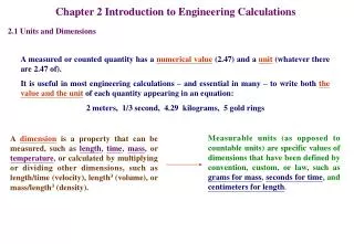
Chapter 2 Introduction to Engineering Calculations. 2.1 Units and Dimensions. A measured or counted quantity has a numerical value (2.47) and a unit (whatever there are 2.47 of). It is useful in most engineering calculations – and essential in many – to write both the

E N D
Chapter 2 Introduction to Engineering Calculations 2.1 Units and Dimensions A measured or counted quantity has a numerical value (2.47) and a unit (whatever there are 2.47 of). It is useful in most engineering calculations – and essential in many – to write both the value and the unit of each quantity appearing in an equation: 2 meters, 1/3 second, 4.29 kilograms, 5 gold rings Measurable units (as opposed to countable units) are specific values of dimensions that have been defined by convention, custom, or law, such as grams for mass, seconds for time, and centimeters for length. A dimension is a property that can be measured, such as length, time, mass, or temperature, or calculated by multiplying or dividing other dimensions, such as length/time (velocity), length3 (volume), or mass/length3 (density).
Units can be treated like algebraic variables when quantities are added, subtracted, multiplied, or divided. The numerical values of two quantities may be added or subtracted only if the units are the same. Numerical values and their corresponding units may always be combined by multiplication or division.
2.2 Conversion of Units To convert a quantity expressed in terms of one unit to its equivalent in terms of another unit, multiply the given quantity by the conversion factor (new unit/old unit). For example, to convert 36 mg to its equivalent in grams, write 1 g 36 mg = 0.036 g 1000 mg If you are given a quantity having a compound unit [e.g., miles/h, cal/(g.C)], and you wish to convert it to its equivalent in terms of another set of units, set up a dimensional equation: write the given quantity and its units on the left, write the units of conversion factors that cancel the old units and replace them with the desired ones, fill in the values of the conversion factors, and carry out the indicated arithmetic to find the desired value. Test Yourself p. 9
Example 2.2-1 Convert an acceleration of 1 cm/s2 to its equivalent in km/yr2. Solution 1 cm 3652 day2 1 m 1 km 36002 s2 242 h2 12 day2 12 yr2 102 cm 12 h2 103 m s2 A principle illustrated in this example is that raising a quantity (in particular, a conversion factor) to a power raises its unit to the same power.
2.3 Systems of Units A system of units has the following components: 1.Base units for mass, length, time, temperature, electrical current, and light intensity. 2.Multiple units, which are defined as multiple or fractions of base units as minutes, hours, and milliseconds, all of which are defined in terms of the base unit of a second. Multiple units are defined for convenience rather than necessity. 3.Derived units, obtained in one of two ways: (a)By multiplying and dividing base or multiple units (cm2, ft/min, kgm/s2, etc.) Derived units of this type are referred to as compound units. (b)As defined equivalents of compound units (e.g., 1 erg 1 gcm2/s2, 1 lbf 32.174 lbmft/s2) Prefixes are used in SI to indicate powers of ten. American engineering system ft (for length), lbm (for mass), s (for time)
Example 2.3-1 Convert 23 lbfft/min2 to its equivalent in kgcm/s2. Solution As before, begin by writing the dimensional equation, fill in the units of conversion factors (new/old) and then the numerical values of these factors, and then do the arithmetic. The result is 23 lbmft 12 min2 0.453593 kg 100 cm (60)2 s2 min2 1 lbm 3.281 ft Test Yourself p. 11
2.4 Force and Weight According to Newton’s second law of motion, force is proportional to the product of mass and acceleration (length/time2). Natural force units are kgm/s2 (SI), gcm/s2 (CGS), lbmft/s2 (American engineering) To avoid having to carry around these complex units in all calculations involving forces, derived force units have been defined in each system. Force in newtons required to accelerate a mass of 4.00 kg at a rate of 9.00 m/s2 Force in lbf required to accelerate a mass of 4.00 lbm at a rate of 9.00 ft/s2 4.00 lbm 1 lbf 4.00 kg 1 N 9.00 ft 9.00 m = 1.12 lbf = 36.0 N F= F= 32.174 lbmft/s2 1 kgm/s2 s2 s2 used to denote the conversion factor from natural to derived force units
The weight of an object is the force exerted on the object by gravitational attraction. Suppose that an object of mass m is subjected to a gravitational force W (W is by definition the weight of the object) and that if this object were falling freely its acceleration would be g. The gravitational acceleration (g) varies directly with the mass of the attracting body (the earth, in most problem you will confront) and inversely with the square of the distance between the centers of mass of the attracting body and the object being attracted. The value of g at sea level and 45 latitude is given below in each system of units: The acceleration of gravity does not vary much with position on the earth’s surface and (within moderate limits) altitude, and the values in this equation may accordingly be used for most conversions between mass and weight. Test Yourself p. 13
Example 2.4-1 Water has a density of 62.4 lbm/ft3. How much does 2.000 ft3 of water weight (1) at sea level and 45 latitude and (2) in Denver, Colorado, where the altitude is 5347 ft and the gravitational acceleration is 32.139 ft/s2 ? Solution The mass of the water is The weight of the water is 1. At sea level g = 32.174 ft/s2, so that W = 124.8 lbf. 2. In Denver, g = 32.139 ft/s2, and W = 124.7 lbf. As this example illustrates, the error incurred by assuming that g = 32.174 ft/s2 is normally quite small as long as you remain on the earth’s surface. In a satellite or on another planet it would be a different story.
2.5 Numerical Calculation and Estimation 2.5a Scientific Notation, Significant Figures, and Precision Both very large and very small numbers are commonly encountered in process calculations. A convenient way to present such numbers is to use scientific notation, in which a number is expressed as the product of another number (usually between 0.1 and 10) and a power of 10. 123,000,000=1.23108 (or 0.123109) 0.000028=2.8 10-5 (or 0.2810-4) The significant figures of a number are the digits from the first nonzero digit on the left to either (a)the last digit (zero or nonzero) on the right if there is a decimal point, or (b)the last nonzero digit of the number if there is no decimal point. 2300 or 2.3103 two significant figures 2300. or 2.300 103 four significant figures 2300.0 or 2.3000 103 five significant figures 23,040 or 2.304 104 four significant figures 0.035 or 3.5 10-2 two significant figures 0.03500 or 3.500 10-2 four significant figures Note: The number of significant figures is easily shown and seen if scientific notation is used.
8.3 g 8.25 and 8.35 g 8.300 g 8.2995 and 8.3005 g The number of significant figures in the reported value of a measured or calculated quantity provides an indication of the precision with which the quantity is known: the more significant figures, the more precise is the value. Generally, if you report the value of a measured quantity with three significant figures, you indicated that the value of the third of these figures may be off by as much as a half-unit. This rule applies only to measured quantities or numbers calculated from measured quantities. If a quantity is known precisely-like a pure integer (2) or a counted rather than measured quantity (16 oranges)-its value implicitly contains an infinite number of significant figure (5 cows really means 5.0000……cows) When two or more quantities are combined by multiplication and/or division, the number of significant figures in the result should equal the lowest number of significant figures of any of the multiplicands or divisors. (3) (4) (7) (3) (3.57)(4.286) = 15.30102 15.3 (2) (4) (3) (9) (2) (2) (5.210-4)(0.1635107)/(2.67) = 318.426966 3.2102 = 320
When two or more numbers are added or subtracted, the positions of the last significant figures of each number relatives to the decimal point should be compared. Of these positions, the one farthest to the left is the position of the last permissible significant of the sum or difference. 1530 -2.56 1.26 1.0000 + 0.036 + 0.22 = 1.2560 1527.44 1530 2.75106 + 3.400104 = (2.75 + 0.03400)106 =2.784000106 2.78106 Finally, a rule of thumb for rounding off numbers in which the digit to be dropped is a 5 is always to make the last digit of the rounded-off number even: 1.35 1.4 1.25 1.2 Test Yourself p. 15
2.5b Validating Results Among approaches you can use to validate a quantitative problem solution are back-substitution, order-of-magnitude estimation, and the test of reasonableness. Back-substitution is straightforward: after you solve a set of equations, substitute your solution back into the equation and make sure it works. Order-of-magnitude estimation means coming up with a crude and easy-to-obtain approximation of the answer to a problem and making sure that the more exact solution comes reasonably close to it. Applying the test of reasonableness means verifying that the solution makes sense. If, for example, a calculated velocity of water flowing in a pipe is faster than the speed of light or the calculated temperature in a chemical reactor is higher than the interior temperature of the sun, you should suspect that a mistake has been made somewhere.
The procedure for checking an arithmetic calculation by order-of-magnitude estimation is as follows: 1.Substitute simple integers for all numerical quantities, using powers of 10 (scientific notation) for very small and very large numbers. 27.36 20 or 30 (whichever makes the subsequent arithmetic easier) 63,472 6104 0.002887 310-3 2.Do the resulting arithmetic calculation by hand, continuing to round off intermediate answers. The correct solution (obtained using a calculator) is 4.78106. If you obtain this solution, since it is of the same magnitude as the estimate, you can be reasonably confident that you haven’t made a gross error in the calculation. 3.If a number is added to a second, much smaller, number, drop the second number in the approximation. The calculator solution is 0.239.
Example 2.5-1 The calculation of a process stream volumetric flow rate has led to the following formula: Solution Estimate without using a calculator. (The exact solution is 0.00230.)
2.5c Estimation of Measured Values: Sample Mean Suppose we carry out a chemical reaction of the form A Product, starting with pure A in the reactor and keeping the reactor temperature at 45 C. After two minutes we draw a sample from the reactor and analyze it to determine X, the percentage of the A fed that has reacted. In theory X should have a unique value; however, in a real reactor X is a random variable, changing in an unpredictable manner from one run to another at the same experimental conditions. The values of X obtained after 10 successive runs might be as follows:
Why don’t we get the same value of X in each run? There are several reasons. ~It is impossible to replicate experimental conditions exactly in successive experiments. If the temperature in the reactor varies by as little as 0.1 degree from one run to another, it could be enough to change the measure value of X. ~Even if conditions were identical in two runs, we could not possibly draw our example at exactly t=2.000… minutes both times, and a difference of a second could make a measurable difference in X. ~Variations in sampling and chemical analysis procedures invariably introduce scatter in measured values. 1. What is the true value of X? In principle there may be such a thing as the “true value”- that is, the value we would measure if we could set the temperature exactly to 45.0000….degrees, start the reaction, keep the temperature and all other experimental variables that affect X perfectly constant, and then sample and analyze with complete accuracy at exactly t=2.0000…minutes. In practice there is no way to do any of those things, however. We could also define the true value of X as the value we would calculate by performing an infinite number of measurement and averaging the results, but there is no practical to do that either. The best we can ever do is to estimate the true value of X from a finite number of measured values.
2. How can we estimate of the true value of X? The most common estimate is the sample mean (or arithmetic mean). We collect N measured value of X (X1, X2, …., XN) and then calculate Sample Mean For the given data, we would estimate Graphically, the data and sample mean might appear as shown right. The measure values scatter about the sample mean, as they must. The more measurements of a random variable, the better the estimated values based on the sample mean. However, even with a huge number of measurements the sample mean is at best an approximation of the true value and could in fact be way off. (e.g., if there is something wrong with the instruments or procedures used to measure X). Test Yourself p. 18
2.5d Sample Variance of Scattered Data Figure 2.5-1 Consider two sets of measurements of a random variable, X – for example, the percentage conversion in the same batch reactor measured using two different experimental techniques. Scatter plots of X versus run number are shown in Figure 2.5-1. The sample mean of each set is 70%, but the measured values scatter over a much narrower range for the first set (from 68% to 73%) than for the second set (from 52% to 95%). In each case you would estimate the true value of X for the given experimental conditions as the sample mean, 70%, but you would clearly have more confidence in the estimate for Set (a) than in that for Set (b). Three quantities – the range, the sample variance, the sample standard deviation – are used to express the extent to which values of a random variable scatter about their mean value.
The range is simple the difference between the highest and lowest values of X in the data set: Figure 2.5-1 Set (a) R=73%-68%=5% Set (b) R=95%-52%=43% The range is the crudest measure of scatter: it involves only two of the measured values and gives no indication of whether or not most of the values cluster close to the mean or scatter widely around it. The sample variance is a much better measure. To define it we calculate the deviation of each measured value from the sample mean, (j=1,2,….,N), and then calculate The degree of scatter may also be expressed in terms of the sample standard deviation, by definition the square root of the sample variance:
The more a measured value (Xj) deviates from the mean, either positively or negatively, the greater the value of and hence the greater the value of the sample variance and sample standard deviation. Figure 2.5-1 Test Yourself p. 19 Figure 2.5-2 For typical random variables, roughly two-thirds of all measured values fall within one standard deviation of the mean; about 95% fall within two standard deviation; and about 99% fall within three standard deviations. The interval between 47.6 and 48.8 may represent the range of the data set (Xmax-Xmin). 0.6 might represent sX, 2sX, 3sX. 27/37 33/37 36/37 error limits
Example 2.5-2 Five hundred batches of a pigment are produced each week. In the plant’s quality assurance (QA) program, each batch is subjected color analysis test. If a batch does not pass the test, it is rejected and sent back for reformulation. Let Y be the number of bad batches produced per week, and suppose that QA test result for a 12-week base period are as follows: The company policy is to regard the process operation as normal as long as the number of bad batches produced in a week is no more than three standard deviations above the mean value for the base period (i.e., as long as ). If Y exceeds this value, the process is shut down for remedial maintenance (a long and costly procedure). Such large deviations from the mean might occur as part of the normal scatter of the process, but so infrequently that if it happens the existence of an abnormal problem in the process is considered the more likely explanation. 1.How many bad batches in a week would it take to shut down the process? 2.What would be the limiting value of Y if two standard deviation instead of three were used as the cutoff criterion? What would be the advantage and disadvantage of using this stricter criterion.
Solution 1. The maximum allowed value of Y is If 29 or more bad batches are produced in a week, the process must be shut down for maintenance. 2. If this criterion were used, 26 bad batches in a week would be enough to shut down the process. The advantage is that if something has gone wrong with the process the problem will be corrected sooner and fewer bad batches will be made in the long run. The disadvantage is that more costly shutdowns may take place when nothing is wrong, the large number of bad batches simply reflecting normal scatter in the process.
2.6 Dimensional Homogeneity and Dimensionless Quantities We began our discussion of units and dimension by saying that quantities can be added and subtracted only if their units are the same. If the units are the same, it follows that the dimensions of each term must be the same. For example, if two quantities can be expressed in terms of grams/second, both must have the dimension (mass/time). This suggests that the following rule: Every valid equation must be dimensionally homogeneous: that is, all additive terms on both sides of the equation must have the same dimensions. dimensionally homogeneous not dimensionally homogeneous The converse of the given rule is not necessarily true – an equation may be dimensionally homogeneous and invalid. For example, if M is the mass of an object, then the equation M=2M is dimensionally homogeneous, but it is also obviously incorrect except for one specific value of M.
Example 2.6-1 Consider the equation 1.If the equation is valid, what are the dimensions of the constants 3 and 4? 2.If the equation is consistent in its units, what are the units of 3 and 4? 3.Derive an equation for distance in meters in terms of time in minutes. Solution 1.The constant 3 must have the dimension (length/time) and 4 must have the dimension (length). 2.For consistency, the constants must be 3 ft/s and 4 ft. 3. D’ (m) 3.2808 ft D(ft)= = 3.28D’ 1 m t’ (min) 60 s = 60t’ t(s)= 1 min
Example 2.6-1 illustrates a general procedure for rewriting an equation in terms of new variable having the same dimensions but different units: 1.Define new variable (e.g., by affixing primes to the old variable names) that have the desired units. 2.Write expression for each old variable in terms of the corresponding new variable. 3.Substitute these expressions in the original equation and simplify. A dimensionless quantity can be a pure number (2, 1.3, 5/2) or a multiplicative combination of variables with no net dimensions: dimensionless group Exponents (such as the 2 in X2), transcendental function (such as log, exp=e, and sin), and arguments of transcendental function (such as the X in sinX) must be dimensionless quantities. 102ft log (20s) sin (3dyne) meaningless
Example 2.6-2 A quantity k depends on the temperature T in the following manner: The units of the quantity 20,000 are cal/mol, and T is in K (kelvin). What are the units of 1.2105 and 1.987? Solution Since the equation must be consistent in its units and exp is dimensionless, 1.2105 should have the same units as k, mol/(cm3s). Moreover, since the argument of exp must be dimensionless, we can write 20,000 cal molK 1 mol T(K) 1.987 cal The answers are thus 1.2105 mol/(cm3s) and 1.987 cal/(molK) Test Yourself p. 22
2.7 Process Data Representation and Analysis The operation of any chemical process is ultimately based on the measurement of process variables – temperatures, pressures, flow rate, concentrations, and so on. It is sometimes possible to measure these variables directly, but, as a rule, indirect techniques must be used. Suppose, for example, that you wish to measure the concentration, C, of a solute in a solution. To do so, you normally measure a quantity, X – such as a thermal or electrical conductivity, a light absorbance, or the volume of a titer – that varies in a known manner with C, and then calculate C from the measured value of X. The relationship between C and X is determined in a separate calibration experiment in which solutions of known concentration are prepared and X is measured for each solution. Consider a calibration experiment in which a variable, y, is measured for several values of another variable, x: Our object is to use the calibration data to estimate the value of y for a value of x between tabulated points (interpolation) or outside the range of the table data (extrapolation). Figure 2.7-1 two point linear interpolation graphical interpolation curve fitting
2.7a Two-Point Linear Interpolation The equation of the line through (x1, y1) and (x2, y2) on a plot of y versus x is You may use this equation to estimate y for an x between x1 and x2. You may also use it to estimate y for an x outside of this range (i.e., to extrapolate the data), but with a much greater risk of inaccuracy. If the points in a table are relatively close together, linear interpolation should provide an accurate estimate of y for any x and vice versa; on the other hand, if the points are widely separated or if the data are to be extrapolated, one of the curve- fitting techniques should be used. Test Yourself p. 23
2.7b Fitting a Straight Line Suppose the values of a dependent variable y have been measured for several values of an independent variable x, and a plot of y versus x on rectangular coordinate axes yields what appears to be a straight line. The equation you would use to represent the relationship between x and y is then (x1, y1) and (x2, y2) are two points – which may or may not be data points – on the line.
Example 2.7-1 Rotameter calibration data (flow rate versus rotameter reading) are as follows: 1.Draw a calibration curve and determine an equation for . 2.Calculate the flow rate that corresponds to a rotameter reading of 36. Solution 1.The calibration curve appears as follows: Check point 2 2.At R=36,
2.7c Fitting Nonlinear Data Fitting a nonlinear equation (anything but y=ax+b) to data is usually much harder than fitting a line; however, with some nonlinear equations you can still use straight-line fitting if you plot the data in a suitable manner. (Quantity 1) = a (Quantity 2) + b Plot y versus x2 Plot 1/y versus x. Slope = C1, intercept = -C2 Plot y2 versus 1/x Plot 1/y versus (x+3) Plot (y-1)2/x2 versus x2. Slope = m, intercept = n Plot siny versus (x2-4) If you have (x, y) data that you wish to fit with an equation that can be written in the form f(x, y)= ag(x, y) + b, 1.Calculate f(x, y) and g(x, y) for each tabulated (x, y) point, and plot f versus g. 2.If the plotted points fall on a straight line, the equation fits the data. Choose two points on the line – (g1, f1) and (g2, f2) – and calculate a and b as
Example 2.7-2 A mass flow rate is measured as a function of temperature T(C). There is reason to believe that varies linearly with the square root of T: Use a straight-line plot to verify this formula and determine a and b. Solution Check point 2
2.7d Logarithmic Coordinates Plot ln y versus x. Slope = b, intercept = ln a Plot ln y versus ln x. Slope = b, intercept = ln a Figure 2.7-2 A plot with logarithmic scale on both axes is called a log plot, and a plot with one logarithmic and one rectangular (equal interval) axis is called a semilog plot. logarithmic scale When you plot values of a variable y on a logarithmic scale you are in effect plotting the logarithm of y on a rectangular scale. Test Yourself p. 27
1.If y versus x data appear linear on a semilog plot, then ln y versus x would be linear on a rectangular plot, and the data can therefore be correlated by an exponential function y = a exp(bx). 2.If y versus x data appear linear on a log plot, then ln y versus ln x would be linear on a rectangular plot, and the data can therefore be correlated by a power law y =axb. 3.When you plot values of a variable z on a logarithmic axis and your plot yields a straight line through two points with coordinate values z1 and z2, replace z2-z1 with ln(z2/z1)(=ln z2-ln z1) in the formula for the slope. 4.Do not plot values of ln z on a logarithmic scale and expect anything useful to result.
Example 2.7-3 A plot of F versus t yields a line that passes through the points (t1=15, F1=0.298) and (t2=30, F2=0.0527) on (1) a semilog plot and (2) a log plot. For each case, calculate the equation that relates F and t. Solution 1.Semilog plot 2.Log plot Test Yourself p. 29
2.7e Fitting a Line to Scattered Data There is little problem fitting a line to data that look like this: A number of statistical techniques exist for fitting a function to a set of scattered data. The application of the most common of these techniques – linear regression or the method of least squares – to the fitting of a straight line to a series of y versus x data points is outlined and illustrated in Appendix A.1. You are much more likely to come up with something more like this: