Bounded Radius Routing
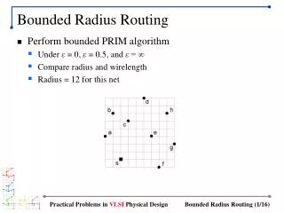
Bounded Radius Routing. Perform bounded PRIM algorithm Under ε = 0, ε = 0.5, and ε = ∞ Compare radius and wirelength Radius = 12 for this net. BPRIM Under ε = 0. Example Edges connecting to nearest neighbors = ( c,d ) and ( c,e ) We choose ( c,d ) based on lexicographical order

Bounded Radius Routing
E N D
Presentation Transcript
Bounded Radius Routing • Perform bounded PRIM algorithm • Under ε = 0, ε = 0.5, and ε = ∞ • Compare radius and wirelength • Radius = 12 for this net Practical Problems in VLSI Physical Design
BPRIM Under ε = 0 • Example • Edges connecting to nearest neighbors = (c,d) and (c,e) • We choose (c,d) based on lexicographical order • s-to-d path length along T = 12+5 > 12 (= radius bound) • First appropriate edge found = (s,d) Practical Problems in VLSI Physical Design
BPRIM Under ε = 0 (cont) • Radius bound = 12 s-to-y path length along T edges connecting to nearest neighbors first feasible appr-edge ties broken lexicographically should be ≤ 12; otherwise appropriate used Practical Problems in VLSI Physical Design
BPRIM Under ε = 0 (cont) Practical Problems in VLSI Physical Design
BPRIM Under ε = 0 (cont) Practical Problems in VLSI Physical Design
BPRIM Under ε = 0.5 • Radius bound = 18 s-to-y path length along T edges connecting to nearest neighbors first feasible appr-edge ties broken lexicographically should be ≤ 18; otherwise appropriate used should be ≤12 Practical Problems in VLSI Physical Design
BPRIM Under ε = 0.5 (cont) Practical Problems in VLSI Physical Design
BPRIM Under ε = 0.5 (cont) Practical Problems in VLSI Physical Design
BPRIM Under ε = ∞ Radius bound = ∞ = regular PRIM Practical Problems in VLSI Physical Design
BPRIM Under ε = ∞ (cont) Practical Problems in VLSI Physical Design
Comparison • As the bound increases (12 → 18 →∞) • Radius value increases (12 →17 → 22) • Wirelength decreases (56 → 49 → 36) Practical Problems in VLSI Physical Design
Bounded Radius Bounded Cost • Perform BRBC under ε = 0.5 • εdefines both radius and wirelength bound • Perform DFS on rooted-MST • Node ordering L = {s, a, b, c, e, f, e, g, e, c, d, h, d, c, b, a, s} • We start with Q = MST Practical Problems in VLSI Physical Design
MST Augmentation • Example: visit a via (s,a) • Running total of the length of visited edges, S = 5 • Rectilinear distance between source and a,dist(s,a) = 5 • We see that ε · dist(s,a) = 0.5 · 5 < S • Thus, we reset S and add (s,a) to Q (note (s,a) is already in Q) Practical Problems in VLSI Physical Design
MST Augmentation (cont) visit nodes based on L dotted edges are added Practical Problems in VLSI Physical Design
Last Step: SPT Computation • Compute rooted shortest path tree on augmented Q Practical Problems in VLSI Physical Design
BPRIM vs BRBC • Under the same ε = 0.5 • BPRIM: radius = 18, wirelength = 49 • BRBC: radius = 12, wirelength = 52 • BRBC: significantly shorter radius at slight wirelength increase Practical Problems in VLSI Physical Design