Using Heuristics in Games
Using Heuristics in Games. At that time two opposing concepts of the game called forth commentary and discussion. The foremost players distinguished two principal types of Game, the formal and the psychological … -- HERMAN HESSE, Magister Ludi (The Glass Bead Game)

Using Heuristics in Games
E N D
Presentation Transcript
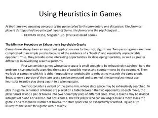
Using Heuristics in Games At that time two opposing concepts of the game called forth commentary and discussion. The foremost players distinguished two principal types of Game, the formal and the psychological … -- HERMAN HESSE, Magister Ludi(The Glass Bead Game) The Minimax Procedure on Exhaustively Searchable Graphs Games have always been an important application area for heuristic algorithms. Two-person games are more complicated than simple puzzles because of the existence of a "hostile“ and essentially unpredictable opponent. Thus, they provide some interesting opportunities for developing heuristics, as weIlas greater difficulties in developing search algorithms. First we consider games whose state space is small enough to be exhaustively searched; here the problem is systematically searching the space of possible moves and countermoves by the opponent. Then we look at games in which it is either impossible or undesirable to exhaustively search the game graph. Because only a portion of the state space can be generated and searched, the game player must use heuristics to guide play along a path to a winning state. We first consider a variant of the game nim, whose state space may be exhaustively searched. To play this game, a number of tokens are placed on a table between the two opponents; at each move, the player must divide a pile of tokens into two nonempty piles of different sizes. Thus, 6 tokens may be divided into piles of 5 and I or 4 and 2, but not 3 and 3. The first player who can no longer make a move loses the game. For a reasonable number of tokens, the state space can be exhaustively searched. Figure 4.19 illustrates the space for a game with 7 tokens.
In playing games whose state space may be exhaustively delineated, the primary difficulty is in accounting for the actions of the opponent. A simple way to handle this assumes that your opponent uses the same knowledge of the state space as you use and applies that knowledge in a consistent effort to win the game. Although this assumption has its limitations (which are discussed in Section 4.3.2), it provides a reasonable basis for predicting an opponent's behavior. Minimax searches the game space under this assumption. The opponents in a game are referred to as MIN and MAX. Although this is partly for historical reasons, the significance of these names is straight forward: MAX represents the player trying to win, or to MAXimize her advantage. MIN is the opponent who attempts to MINimize MAX's score. We assume that MIN uses the same information and always attempts to move to a state that is worst for MAX. In implementing minimax, we label each level in the search space according to whose move it is at that point in the game, MIN or MAX. In the example of Figure 4.20, MIN is allowed to move first. Each leaf node is given a value of I or 0, depending on whether it is a win for MAX or for MIN. Minimax propagates these values up the graph through successive parent nodes according to the rule: If the parent state is a MAX node, give it the maximum value among its children. If the parent is a MIN node, give it the minimum value of its children. The value that is thus assigned to each state indicates the value of the best state that this player can hope to achieve (assuming the opponent plays as predicted by the minimax algorithm). These derived values are used to choose among possible moves. The result of applying minimax to the state space graph for nim appears in Figure 4.20. The values of the leaf nodes are propagated up the graph using minimax. Because all of MIN's possible first moves lead to nodes with a derived value of I, the second player, MAX, always can force the game to a win, regardless of MIN's first move. MIN could win only if MAX played foolishly. In Figure 4.20, MIN may choose any of the first move alternatives, with the resulting win paths for MAX in bold arrows.
Although there are games where it is possible to search the state space exhaustively, most interesting games do not. We examine the fixed depth search next. Minimaxing to Fixed Ply Depth In applying minimax to more complicated games, it is seldom possible to expand the state space graph out to the leaf nodes. Instead, the state space is searched to a predefined number of levels, as determined by available resources of time and memory. This strategy is called an n-ply look-ahead, where n is the number of levels explored. As the leaves of this subgraph are not final states of the game, it is not possible to give them values that reflect a win or a loss. Instead each node is given a value according to some heuristic evaluation function. The value that is propagated back to the root node is not an indication of whether or not a win can be achieved (as in the previous example) but is simply the heuristic value of the best state that can be reached in n moves from the root. Look-ahead increases the power of a heuristic by allowing it to be applied over a greater area of the state space. Minimax consolidates these separate evaluations for the ancestor state. In a game of conflict, each player attempts to overcome the other, so many game heuristics directly measure the advantage of one player over another. In checkers or chess, piece advantage is important, so a simple heuristic might take the difference in the number of pieces belonging to MAX and MIN and try to maximize the difference between these piece measures. A more sophisticated strategy might assign different values to the pieces, depending on their value (e.g., queen vs. pawn or king vs. ordinary checker) or location on the board. Most games provide limitless opportunities for designing heuristics. Game graphs are searched by level, or ply. As we saw in Figure 4.20, MAX and MIN alternately select moves. Each move by a player defines a new ply of the graph. Game playing programs typically look ahead a fixed ply depth, often determined by the space/time limitations of the computer. The states on that ply are measured heuristically and the values are propagated back up the graph using minimax. The search algorithm then uses these derived values to select among possible next moves.
After assigning an evaluation to each state on the selected ply, the program propagates a value up to each parent state. If the parent is on a MIN level, the minimum value of the children is backed up. If the parent is a MAX node, minimax assigns it the maximum value of its children. Maximizing for MAX parents and minimizing for MIN, the values go back up the graph to the children of the current state. These values are then used by the current state to select among its children. Figure 4.21 shows minimax on a hypothetical state space with a four-ply look-ahead. We can make several final points about the minimax procedure. First, and most important, evaluations to any (previously decided) fixed ply depth may be seriously misleading. When a heuristic is applied with limited look-ahead, it is possible the depth of the look-ahead may not detect that a heuristically promising path leads to a bad situation later in the game. If your opponent in chess offers a rook as a lure to take your queen, and the evaluation only looks ahead to the ply where the rook is offered, the evaluation is going to be biased toward this state. Unfortunately, selection of the state may cause the entire game to be lost! This is referred to as the horizon effect. It is usually countered by searching several plies deeper from states that look exceptionally good. This selective deepening of search in important areas will not make the horizon effect go away, however. The search must stop somewhere and will be blind to states beyond that point. There is another effect that occurs in minimaxing on the basis of heuristic evaluations. The evaluations that take place very deep in the space can be biased by their very depth (Pearl 1984). In the same way that the average of products differs from the product of averages, the estimate of minimax (which is what we desire) is different from the minimax of estimates (which is what we are doing). In this sense, deeper search with evaluation and minimax normally does, but need not always, mean better search. Further discussion of these issues and possible remedies may be found in Pearl (1984). In concluding the discussion of minimax, we present an application to tic-tac-toe (Section 4.0), adapted from Nilsson (1980). A slightly more complex heuristic is used, one that attempts to measure the conflict in the game. The heuristic takes a state that is to be measured, counts all winning lines open to MAX, and then subtracts the total number of winning lines open to MIN.
The search attempts to maximize this difference. If a state is a forced win for MAX, it is evaluated as +∞; a forced win for MIN, as -∞. Figure 4.22 shows this heuristic applied to several sample states. Figures 4.23. 4.24, and 4.25 demonstrate the heuristic of Figure 4.22 in a two-ply minimax. These figures show the heuristic evaluation, minimax backup, and MAX's move, with some type of tiebreaker applied to moves of equal value, from Nilsson (1971). The Alpha-Beta Procedure Straight minimax requires a two-pass analysis of the search space, the first to descend to the ply depth and there apply the heuristic and the second to propagate values back up the tree. Minimax pursues all branches in the space, including many that could be ignored or pruned by a more intelligent algorithm. Researchers in game playing developed a class of search techniques called alpha-beta pruning, first proposed in the late 1950s (Newell and Simon 1976), to improve search efficiency in two-person games (Pearl 1984). The idea for alpha-beta search is simple: rather than searching the entire space to the ply depth, alpha-beta search proceeds in a depth-first fashion. Two values, called alpha and beta, are created during the search. The alpha value, associated with MAX nodes, can never decrease, and the beta value, associated with MIN nodes, can never increase. Suppose a MAX node's alpha value is 6. Then MAX need not consider any backed-up value less than or equal to 6 that is associated with any MIN node below It. Alpha is the worst that MAX can "score" given that MIN will also do its "best." Similarly, if MIN has beta value 6, it does not need to consider any MAX node below that has a value of 6 or more. To begin alpha-beta search, we descend to full ply depth in a depth-first fashion and apply our heuristic evaluation to a state and all its siblings. Assume these are MIN nodes. The maximum of these MIN values is then backed up to the parent (a MAX node, just as in minimax). This value is then offered to the grandparent of these MINs as a potential beta cutoff. Next, the algorithm descends to other grandchildren and terminates exploration of their parent if any of their values is equal to or larger than this beta value. Similar procedures can be described for alpha pruning over the grandchildren of a MAX node. Two rules for terminating search, based on alpha and beta values, are: Search can be stopped below any MIN node having a beta value less than or equal to the alpha value of any of its MAX ancestors. Search can be stopped below any MAX node having an alpha value greater than or equal to the beta value of any of its MIN node ancestors.
Alpha-beta pruning thus expresses a relation between nodes at ply n and nodes at ply n + 2 under which entire subtrees rooted at level n + 1 can be eliminated from consideration. As an example, Figure 4.26 takes the space of Figure 4.21 and applies alpha-beta pruning. Note that the resulting backed-up value is identical to the minimaxresult and the search saving over minimax is considerable. With a fortuitous ordering of states in the search space, alpha-beta can effectively double the depth of the search space considered with a fixed space/time computer commitment (Nilsson 1980). If there is a particular unfortunate ordering, alpha-beta searches no more of the space than normal minimax; however, the search is done in only one pass. Complexity Issues The most difficult aspect of combinatorial problems is that the "explosion" often takes place without program designers realizing that it is happening. Because most human activity, computational and otherwise, takes place in a linear-time world, we have difficulty appreciating exponential growth. We hear the complaint: "If only I had a larger (or faster or highly parallel) computer my problem would be solved." Such claims, often made in the aftermath of the explosion, are usually rubbish. The problem wasn't understood properly and/or appropriate steps were not taken to address the combinatorics of the situation. The full extent of combinatorial growth staggers the imagination. It has been estimated that the number of states produced by a full search of the space of possible chess moves is about 10120, This is not “just another large number;” it is comparable to the number of molecules in the universe or the number of nanoseconds since the “big bang.”
Several measures have been developed to help calculate complexity. One of these is the Branching factor of a space. We define branching factor as the average number of branches (children) that are expanded from any state in the space. The number of states at depth n of the search is equal to the branching factor raised to the nth power. Once the branching factor is computed for a space it is possible to estimate the search cost to generate a path of any particular length. Figure 4.27 gives the relationship between B (branching), L (path length), and T (total states in the search) for small values. The figure is logarithmic in T, so L is not the straight line it looks in the graph. Several examples using this figure show how bad things can get. If the branching factor is 2 (in a binary tree, for example), it takes a search of about 100 states to examine all paths that extend six levels deep into the search space. It takes a search of about 10,000 states to consider paths 12 moves deep. If the branching can be cut down to 1.5 (by some heuristic or reformulation of the problem), then a path twice as long can be examined for the same number of states searched. The mathematical formula that produced the relationships of Figure 4.27 is: T = B + B2+ B3+ … + BL with T is total states, L is path length, and B is branching factor. This equation reduces to: T = B (BL- 1)/(B - 1) Measuring a search space is usually an empirical process done by considerable playing with a problem and testing its variants. Suppose, for example, we wish to establish the branching factor of the 8-puzzle. We calculate the total number of possible moves: 2 from each corner for a total of 8 corner moves, 3 from the center of each side for a total of 12, and 4 from the center of the grid for a grand total of 24. This divided by 9, the different number of possible locations of the blank, gives an average branching factor of 2.67. As can be seen in Figure 4.27, this is not very good for a deep search. If we eliminate moves directly back to a parent state (already built into the search algorithms of this chapter) there is one move fewer from each state. This gives a branching factor of 1.67, a considerable improvement, which might (in some state spaces) make exhaustive search possible.
As we considered in Chapter 3, the complexity cost of an algorithm can also be measured by the sizes of the open and closed lists. One method of keeping the size of open reasonable is to save on open only a few of the (heuristically) best states. This can produce a better focused search but has the danger of possibly eliminating the best, or even the only, solution path. This technique of maintaining a size bound, often a function of the number of steps taken in the search, is called beam search. In the attempt to bring down the branching of a search or otherwise constrain the search space, we presented the notion of more informed heuristics. The more informed the search, the less the space must be searched to get the minimal path solution. As we pointed out in Section 4.3, the computational costs of the additional information needed to further cut down the search space may not always be acceptable. In solving problems on a computer, it is not enough to find a minimum path. We must also minimize total cpu costs. Figure 4.28, taken from an analysis by Nilsson (1980), is an informal attempt to get at these issues. The "informedness" coordinate marks the amount of information costs that are included in the evaluation heuristic that are intended to improve performance. The cpu coordinate marks the cpu costs for implementing state evaluation and other aspects of the search. As the information included in the heuristic increases, the cpu cost of the heuristic increases. Similarly, as the heuristic gets more informed, the cpu cost of evaluating states gets smaller, because fewer states are considered. The critical cost, however, is the total cost of computing the heuristic PLUS evaluating states, and it is usually desirable that this cost be minimized. Finally, heuristic search of and/or graphs is an important area of concern, as the state spaces for expert systems are often of this form. The fully general search of these structures is made up of many of the components already discussed in this and the preceding chapter. Because all and children must be searched to find a goal, the heuristic estimate of the cost of searching an and node is the sum of the estimates of searching the children.
There are many further heuristic issues, however, besides the numerical evaluation of individual and states, in the study of and/or graphs, such as are used in knowledge based systems. For instance, if the satisfaction of a set of and children is required for solving a parent state, which child should be considered first? The state most costly to evaluate? The state most likely to fail? The state the human expert considers first? The decision is important both for computational efficiency as well as overall cost, e.g., in medical or other diagnostic tests, of the knowledge system. These, as well as other related heuristic issues, are visited again in Chapter 8.