Intermediate Representations
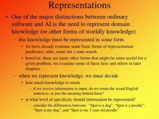
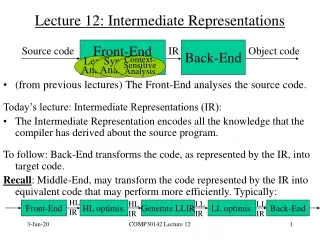
Intermediate Representations. Source Code. Front End. Middle End. Back End. IR. IR. Target Code. Intermediate Representations. Front end - produces an intermediate representation ( IR ) Middle end - transforms the IR into an equivalent IR that runs more efficiently

Intermediate Representations
E N D
Presentation Transcript
Source Code Front End Middle End Back End IR IR Target Code Intermediate Representations • Front end - produces an intermediate representation (IR) • Middle end - transforms the IR into an equivalent IR that runs more efficiently • Back end - transforms the IR into native code • IR encodes the compiler’s knowledge of the program • Middle end usually consists of several passes
Intermediate Representations • Decisions in IR design affect the speed and efficiency of the compiler • Some important IR properties • Ease of generation • Ease of manipulation • Procedure size • Freedom of expression • Level of abstraction • The importance of different properties varies between compilers • Selecting an appropriate IR for a compiler is critical
Types of Intermediate Representations Three major categories • Structural • Graphically oriented • Heavily used in source-to-source translators • Tend to be large • Linear • Pseudo-code for an abstract machine • Level of abstraction varies • Simple, compact data structures • Easier to rearrange • Hybrid • Combination of graphs and linear code • Example: control-flow graph Examples: Trees, DAGs Examples: 3 address code Stack machine code Example: Control-flow graph
subscript j A i Level of Abstraction • The level of detail exposed in an IR influences the profitability and feasibility of different optimizations. • Two different representations of an array reference: loadI 1 => r1 sub rj, r1 => r2 loadI 10 => r3 mult r2, r3 => r4 sub ri, r1 => r5 add r4, r5 => r6 loadI @A => r7 Add r7, r6 => r8 load r8 => rAij High level AST: Good for memory disambiguation Low level linear code: Good for address calculation
load Low level AST loadArray A,i,j @A j j High level linear code - - + * + 10 1 1 Level of Abstraction • Structural IRs are usually considered high-level • Linear IRs are usually considered low-level • Not necessarily true:
* x - y 2 Abstract Syntax Tree An abstract syntax tree is the procedure’s parse tree with the nodes for most non-terminal nodes removed x - 2 * y • Can use linearized form of the tree • Easier to manipulate than pointers x 2 y * - in postfix form - * 2 y x in prefix form • S-expressions are (essentially) ASTs
/ z w * x y 2 - Directed Acyclic Graph A directed acyclic graph (DAG) is an AST with a unique node for each value • Makes sharing explicit • Encodes redundancy z x - 2 * y w x / 2
Stack Machine Code Originally used for stack-based computers, now Java • Example: x - 2 * y becomes Advantages • Compact form • Introduced names are implicit, not explicit • Simple to generate and execute code Useful where code is transmitted over slow communication links (the net) push x push 2 push y multiply subtract Implicit names take up no space, where explicit ones do!
Three Address Code Several different representations of three address code • In general, three address code has statements of the form: x y op z With 1 operator (op) and, at most, 3 names (x, y, & z) Example: z x - 2 * y becomes Advantages: • Resembles many machines • Introduces a new set of names • Compact form t 2 * y z x - t
Three Address Code: Quadruples Naïve representation of three address code • Table of k * 4 small integers • Simple record structure • Easy to reorder • Explicit names The original FORTRAN compiler used “quads” load r1, y loadI r2, 2 mult r3, r2, r1 load r4, x sub r5, r4, r3 RISC assembly code Quadruples
(1) (2) (3) (4) (5) Three Address Code: Triples • Index used as implicit name • 25% less space consumed than quads • Much harder to reorder Implicit names take no space!
Three Address Code: Indirect Triples • List first triple in each statement • Implicit name space • Uses more space than triples, but easier to reorder • Major tradeoff between quads and triples is compactness versus ease of manipulation • In the past compile-time space was critical • Today, speed may be more important (100) (100) (105) (101) (102) (103) (104)
Static Single Assignment Form • The main idea: each name defined exactly once • Introduce -functions to make it work Strengths of SSA-form • Sharper analysis • -functions give hints about placement Original x … y … while (x < k) x x + 1 y y + x SSA-form x0 … y0 … if (x0 > k) goto next loop: x1 (x0,x2) y1 (y0,y2) x2 x1 + 1 y2 y1 + x2 if (x2 < k) goto loop next: …
Two Address Code • Allows statements of the form x x op y Has 1 operator (op) and, at most, 2 names (x and y) Example: z x - 2 * y becomes • Can be very compact Problems • Machines no longer rely on destructive operations • Difficult name space • Destructive operations make reuse hard • Good model for machines with destructive ops (PDP-11) t1 2 t2 load y t2 t2 * t1 z load x z z - t2
if (x = y) Basic blocks — Maximal length sequences of straight-line code a 2 b 5 a 3 b 4 c a * b Control-flow Graph Models the transfer of control in the procedure • Nodes in the graph are basic blocks • Can be represented with quads or any other linear representation • Edges in the graph represent control flow Example
Source Code Front End IR 1 Middle End IR 2 Middle End IR 3 Back End Target Code Using Multiple Representations • Repeatedly lower the level of the intermediate representation • Each intermediate representation is suited towards certain optimizations • Example: the Open64 compiler • WHIRL intermediate format • Consists of 5 different IRs that are progressively more detailed
Memory Models Two major models • Register-to-register model • Keep all values that can legally be stored in a register in registers • Ignore machine limitations on number of registers • Compiler back-end must insert loads and stores • Memory-to-memory model • Keep all values in memory • Only promote values to registers directly before they are used • Compiler back-end can remove loads and stores • Compilers for RISC machines usually use register-to-register • Reflects programming model • Easier to determine when registers are used
The Rest of the Story… Representing the code is only part of an IR There are other necessary components • Symbol table (already discussed) • Constant table • Representation, type • Storage class, offset • Storage map • Overall storage layout • Overlap information • Virtual register assignments
The Procedure as a Control Abstraction Procedures have well-defined control-flow The Algol-60 procedure call • Invoked at a call site, with some set of actual parameters • Control returns to call site, immediately after invocation
The Procedure as a Control Abstraction Procedures have well-defined control-flow The Algol-60 procedure call • Invoked at a call site, with some set of actual parameters • Control returns to call site, immediately after invocation int p(a,b,c) int a, b, c; { int d; d = q(c,b); ... } … s = p(10,t,u); …
The Procedure as a Control Abstraction Procedures have well-defined control-flow The Algol-60 procedure call • Invoked at a call site, with some set of actual parameters • Control returns to call site, immediately after invocation int p(a,b,c) int a, b, c; { int d; d = q(c,b); ... } int q(x,y) int x,y; { return x + y; } … s = p(10,t,u); …
The Procedure as a Control Abstraction Procedures have well-defined control-flow The Algol-60 procedure call • Invoked at a call site, with some set of actual parameters • Control returns to call site, immediately after invocation int p(a,b,c) int a, b, c; { int d; d = q(c,b); ... } int q(x,y) int x,y; { return x + y; } … s = p(10,t,u); …
The Procedure as a Control Abstraction Procedures have well-defined control-flow The Algol-60 procedure call • Invoked at a call site, with some set of actual parameters • Control returns to call site, immediately after invocation int p(a,b,c) int a, b, c; { int d; d = q(c,b); ... } int q(x,y) int x,y; { return x + y; } … s = p(10,t,u); …
The Procedure as a Control Abstraction Procedures have well-defined control-flow The Algol-60 procedure call • Invoked at a call site, with some set of actual parameters • Control returns to call site, immediately after invocation • Most languages allow recursion int p(a,b,c) int a, b, c; { int d; d = q(c,b); ... } int q(x,y) int x,y; { return x + y; } … s = p(10,t,u); …
int p(a,b,c) int a, b, c; { int d; d = q(c,b); ... } int q(x,y) int x,y; { return x + y; } … s = p(10,t,u); … The Procedure as a Control Abstraction Implementing procedures with this behavior • Requires code to save and restore a “return address” • Must map actual parameters to formal parameters(cx, by) • Must create storage for local variables (&, maybe, parameters) • p needs space for d (&, maybe, a, b, & c) • where does this space go in recursive invocations? Compiler emits code that causes all this to happen at run time
int p(a,b,c) int a, b, c; { int d; d = q(c,b); ... } int q(x,y) int x,y; { return x + y; } … s = p(10,t,u); … The Procedure as a Control Abstraction Implementing procedures with this behavior • Must preserve p’s state while q executes • recursion causes the real problem here • Strategy: Create unique location for each procedure activation • Can use a “stack” of memory blocks to hold local storage and return addresses Compiler emits code that causes all this to happen at run time
The Procedure as a Name Space Each procedure creates its own name space Any name (almost) can be declared locally Local names obscure identical non-local names Local names cannot be seen outside the procedure Nested procedures are “inside” by definition We call this set of rules & conventions “lexical scoping” Examples C has global, static, local, and block scopes (Fortran-like) Blocks can be nested, procedures cannot Scheme has global, procedure-wide, and nested scopes (let) Procedure scope (typically) contains formal parameters
The Procedure as a Name Space Why introduce lexical scoping? Provides a compile-time mechanism for binding “free” variables Simplifies rules for naming & resolves conflicts How can the compiler keep track of all those names? The Problem At point p, which declaration of x is current? At run-time, where is x found? As parser goes in & out of scopes, how does it delete x? The Answer Lexically scoped symbol tables (see § 5.7.3)
Do People Use This Stuff ? C macro from the MSCP compiler #define fix_inequality(oper, new_opcode) \ if (value0 < value1) \ { \ Unsigned_Int temp = value0; \ value0 = value1; \ value1 = temp; \ opcode_name = new_opcode; \ temp = oper->arguments[0]; \ oper->arguments[0] = oper->arguments[1]; \ oper->arguments[1] = temp; \ oper->opcode = new_opcode; \ } Declares a new name
Do People Use This Stuff ? C code from the MSCP implementation More local declarations! static Void phi_node_printer(Block *block) { Phi_Node *phi_node; Block_ForAllPhiNodes(phi_node, block) { if (phi_node->old_name < register_count) { Unsigned_Int i; fprintf(stderr, "Phi node for r%d: [", phi_node->old_name); for (i = 0; i < block->pred_count; i++) fprintf(stderr, " r%d", phi_node->parms[i]); fprintf(stderr, " ] => r%d\n", phi_node->new_name); } else { Unsigned_Int2 *arg_ptr; fprintf(stderr, "Phi node for %s: [", Expr_Get_String(Tag_Unmap( phi_node->old_name))); Phi_Node_ForAllParms(arg_ptr, phi_node) fprintf(stderr, " %d", *arg_ptr); fprintf(stderr, " ] => %d\n", phi_node->new_name); } } }
Lexically-scoped Symbol Tables The problem The compiler needs a distinct record for each declaration Nested lexical scopes admit duplicate declarations The interface insert(name, level ) – creates record for name at level lookup(name, level ) – returns pointer or index delete(level ) – removes all names declared at level Many implementation schemes have been proposed (see § B.4) We’ll stay at the conceptual level Hash table implementation is tricky, detailed, & fun § 5.7 in EaC Symbol tables are compile-time structures the compiler use to resolve references to names. We’ll see the corresponding run-time structures that are used to establish addressability later.
Example procedure p { int a, b, c procedure q { int v, b, x, w procedure r { int x, y, z …. } procedure s { int x, a, v … } … r … s } … q … } B0: { int a, b, c B1: { int v, b, x, w B2: { int x, y, z …. } B3: { int x, a, v … } … } … }
Lexically-scoped Symbol Tables High-level idea Create a new table for each scope Chain them together for lookup ... p a q r b x • v ... c b y x w z • “Sheaf of tables” implementation • insert() may need to create table • it always inserts at current level • lookup() walks chain of tables & • returns first occurrence of name • delete() throws away table for level • p, if it is top table in the chain • If the compiler must preserve the table (for,say,thedebugger),this idea is actually practical. • Individual tables can be hash tables.
Implementing Lexically Scoped Symbol Tables Stack organization • Implementation • insert () creates new level pointer if needed and inserts at nextFree • lookup () searches linearly from nextFree–1 forward • delete () sets nextFree to the equal the start location of the level deleted. • Advantage • Uses much less space • Disadvantage • Lookups can be expensive growth nextFree z y r (level 2) x w x b q (level 1) v c b p (level 0) a
Implementing Lexically Scoped Symbol Tables Threaded stack organization • Implementation • insert () puts new entry at the head of the list for the name • lookup () goes direct to location • delete () processes each element in level being deleted to remove from head of list • Advantage • lookup is fast • Disadvantage • delete takes time proportional to number of declared variables in level • growth • • z y h(x) • x r w • x b q v c b p • a
The Procedure as an External Interface OS needs a way to start the program’s execution Programmer needs a way to indicate where it begins The “main” procedure in most languaages When user invokes “grep” at a command line OS finds the executable OS creates a process and arranges for it to run “grep” “grep” is code from the compiler, linked with run-time system Starts the run-time environment & calls “main” After main, it shuts down run-time environment & returns When “grep” needs system services It makes a system call, such as fopen() UNIX/Linux specific discussion
Where Do All These Variables Go? Automatic & Local • Keep them in the procedure activation record or in a register • Automatic lifetime matches procedure’s lifetime Static • Procedure scope storage area affixed with procedure name • &_p.x • File scope storage area affixed with file name • Lifetime is entire execution Global • One or more named global data areas • One per variable, or per file, or per program, … • Lifetime is entire execution
C o d e S G t l a & o t b i a c l H e a p S t a c k high 0 Single Logical Address Space Placing Run-time Data Structures Classic Organization • Better utilization if • stack & heap grow • toward each other • Very old result (Knuth) • Code & data separate or • interleaved • Uses address space, • not allocated memory • Code, static, & global data have known size • Use symbolic labels in the code • Heap & stack both grow & shrink over time • This is a virtual address space
C o d e C o d e C o d e C o d e S G t l a & o t b i a c l S G t l a & o t b i a c l S G t l a & o t b i a c l S G t l a & o t b i a c l H e a p H e a p H e a p H e a p S t a c k S t a c k S t a c k S t a c k ... How Does This Really Work? The Big Picture virtual address spaces Compiler’s view OS’s view ... 0 high Physical address space_ Hardware’s view
Where Do Local Variables Live? A Simplistic model Allocate a data area for each distinct scope One data area per “sheaf” in scoped table What about recursion? Need a data area per invocation (or activation) of a scope We call this the scope’s activation record The compiler can also store control information there ! More complex scheme One activation record (AR) per procedure instance All the procedure’s scopes share a single AR(may share space) Static relationship between scopes in single procedure Used this way, “static” means knowable at compile time (and, therefore, fixed).
Translating Local Names How does the compiler represent a specific instance of x ? Name is translated into a static coordinate < level,offset > pair “level” is lexical nesting level of the procedure “offset” is unique within that scope Subsequent code will use the static coordinate to generate addresses and references “level” is a function of the table in which x is found Stored in the entry for each x “offset” must be assigned and stored in the symbol table Assigned at compile time Known at compile time Used to generate code that executes at run-time
Storage for Blocks within a Single Procedure • Fixed length data can always be at a constant offset from the beginning of a procedure • In our example, the a declared at level 0 will always be the first data element, stored at byte 0 in the fixed-length data area • The x declared at level 1 will always be the sixth data item, stored at byte 20 in the fixed data area • The x declared at level 2 will always be the eighth data item, stored at byte 28 in the fixed data area • But what about the a declared in the second block at level 2? B0: { int a, b, c B1: { int v, b, x, w B2: { int x, y, z …. } B3: { int x, a, v … } … } … }
Arrays If size is fixed at compile time, store in fixed-length data area If size is variable, store descriptor in fixed length area, with pointer to variable length area Variable-length data area is assigned at the end of the fixed length area for block in which it is allocated Variable-length Data B0: { int a, b … assign value to a B1: { int v(a), b, x B2: { int x, y(8) …. } a b v b x x y(8) v(a) Variable-length data Includes variable length data for all blocks in the procedure …
Activation Record Basics parameters register save area return value return address addressability ARP caller’s ARP local variables Space for parameters to the current routine Saved register contents If function, space for return value Address to resume caller Help with non-local access To restore caller’s AR on a return Space for local values & variables (including spills) One AR for each invocation of a procedure
Activation Record Details How does the compiler find the variables? They are at known offsets from the AR pointer The static coordinate leads to a “loadAI” operation Level specifies an ARP, offset is the constant Variable-length data If AR can be extended, put it below local variables Leave a pointer at a known offset from ARP Otherwise, put variable-length data on the heap Initializing local variables Must generate explicit code to store the values Among the procedure’s first actions
Activation Record Details Where do activation records live? If lifetime of AR matches lifetime of invocation, AND If code normally executes a “return” Keep ARs on a stack If a procedure can outlive its caller, OR If it can return an object that can reference its execution state ARs must be kept in the heap If a procedure makes no calls AR can be allocated statically Efficiency prefers static, stack, then heap C o d e S G t l a & o t b i a c l H e a p S t a c k Yes! This stack.
Communicating Between Procedures Most languages provide a parameter passing mechanism • Expression used at “call site” becomes variable in callee Two common binding mechanisms • Call-by-reference passes a pointer to actual parameter • Requires slot in the AR (for address of parameter) • Multiple names with the same address? • Call-by-value passes a copy of its value at time of call • Requires slot in the AR • Each name gets a unique location (may have same value) • Arrays are mostly passed by reference, not value • Can always use global variables … call fee(x,x,x);
{ Must find the right AR Need links to nameable ARs Establishing Addressability Must create base addresses • Global & static variables • Construct a label by mangling names (i.e., &_fee) • Local variables • Convert to static data coordinate and use ARP + offset • Local variables of other procedures • Convert to static coordinates • Find appropriate ARP • Use that ARP + offset
parameters register save area parameters parameters register save area register save area return value return value return value return address return address return address access link access link access link ARP caller’s ARP caller’s ARP caller’s ARP local variables local variables local variables Establishing Addressability Using access links • Each AR has a pointer to AR of lexical ancestor • Lexical ancestor need not be the caller • Reference to <p,16> runs up access link chain to p • Cost of access is proportional to lexical distance Some setup cost on each call