Download
1 / 54
540 likes | 763 Vues
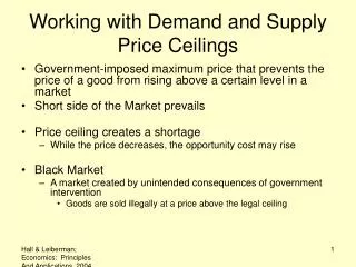
Working with Demand and Supply Price Ceilings. Government-imposed maximum price that prevents the price of a good from rising above a certain level in a market Short side of the Market prevails Price ceiling creates a shortage While the price decreases, the opportunity cost may rise

E N D
Working with Demand and Supply Price Ceilings • Government-imposed maximum price that prevents the price of a good from rising above a certain level in a market • Short side of the Market prevails • Price ceiling creates a shortage • While the price decreases, the opportunity cost may rise • Black Market • A market created by unintended consequences of government intervention • Goods are sold illegally at a price above the legal ceiling
5. With a black market, the lowerquantity sells for a higher price than initially. 4. The result is a shortage – the distance between R and V. Price per Bottle 3. and decreases quantity supplied. 2. increases quantity demanded 1. A price ceiling lowerthan the equilibrium price . . . Number of Bottles of Maple Syrup per Period Figure 1: A Price Ceiling in the Market for Maple Syrup S T $4.00 E 3.00 R V 2.00 D 40,000 50,000 60,000
Price Floors • Government imposed minimum amount below which price is not permitted to fall • Price floors for agricultural goods are commonly called price support programs • When sellers produce more of the good than buyers want at the price floor • Remaining goods become a surplus that no one wants at the imposed price • Government responds by maintaining price floors • Uses taxpayer dollars to buy up entire excess supply of the good in question • Prevents excess supply from doing what it would ordinarily do • Drive price down to its equilibrium value
2. decreases quantity demanded . . . Price per Pound 3. and increases quantity supplied. 1. A price floor higher than the equilibrium price . . . 4. The result is a surplus the – distance between K and J – which government must buy. Millions of Pounds Figure 2: A Price Floor in the Market for Nonfat Dry Milk S J K $0.81 A 0.65 D 180 200 220
Limiting Surplus • A price floor creates a surplus of goods • In order to maintain price floor, government must prevent surplus from driving down market price • Government often accomplishes this goal by purchasing surplus with taxpayers dollars • Price floors often get government deeply involved in production decisions • Rather than leaving them to the market
Supplier’s perspective • A producer considers increasing his price • Is it a good idea? • Higher price means more revenue per unit output BUT… • Lower units of quantity sold (downward sloping demand).
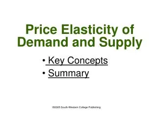
The Problem with Rate Change • Rate of change of quantity demanded compared to the change in price is not a good measure of price sensitivity • Doesn’t tell whether a change in price or a change in quantity demanded is a relatively large or relatively small change • Relative means compared to value of price or quantity before change
The Elasticity Approach • Elasticity approach improves on the problems with rate of change • By comparing percentage change in quantity demanded with percentage change in price • Price elasticity of demand (ED) for a good is percentage change in quantity demanded divided by percentage change in price • Will virtually always be a negative number • Tells us percentage change in quantity demanded for each 1% increase in price • Price elasticity of demand tells us percentage change in quantity demanded caused by a 1% rise in price as we move along a demand curve from one point to another
Calculating Price Elasticity of Demand • When calculating elasticity base value for percentage changes in price or quantity is always midway between initial value and new value • When price changes from any value P0 to any other value P1, we define the percentage change in price as • When quantity demanded changes from Q0 to Q1, percentage change is calculated as
Price per Laptop D $3,500 C 3,000 2,500 2,000 B 1,500 A 1,000 D 100,000 200,000 300,000 400,000 500,000 600,000 Quantity of Laptops Figure 3: Calculating Price Elasticity of Demand
An Example: Calculating Price Elasticity of Demand • Now let’s calculate an elasticity of demand for laptop computers using data in Figure 3 from point A to point B • Use percentage changes for price and quantity to calculate price elasticity of demand (ED)
Elasticity and Straight-Line Demand Curves • As we move upward and leftward along a straight-line demand curve • Same absolute increment in price will correspond to smaller and smaller percentage increments in price • Why? • As we move upward and leftward along a straight-line demand curve • Same absolute decrease in quantity corresponds to larger and larger percentage decreases in quantity • As we move upward and leftward by equal distances, percentage change in quantity rises • Percentage change in price falls • Elasticity of demand varies along a straight-line demand curve • Demand becomes more elastic as we move upward and leftward
Since equal dollar increases (vertical arrows) are smaller and smaller percentage increases . . . Price and since equal quantity decreases (horizontal arrows) are larger and larger percentage decreases . . . demand becomes more and more elastic as we move leftward and upward along a straight-line demand curve. Quantity Figure 4: Elasticity and Straight-Line Demand Curves 3 2 1 D
Categorizing Goods by Elasticity • Inelastic Demand • Price elasticity of demand between 0 and -1 |% Change in Quantity Demanded| < |% Change in Price| • Perfectly Inelastic Demand • Price elasticity of demand equal to 0
Categorizing Goods by Elasticity • Elastic Demand • Price elasticity of demand with absolute value > 1 |% Change in Quantity Demanded| > |% Change in Price| • Perfectly (infinitely) Elastic Demand • Price elasticity of demand approaching minus infinity • Unitary Elastic Demand • Price elasticity of demand equal to -1
(a) Price per Unit Price per Unit $4 $4 Perfectly Elastic Demand 3 3 Perfectly Inelastic Demand 2 2 1 1 20 40 60 80 100 20 40 60 80 100 Quantity Quantity Figure 5: Extreme Cases of Demand (b) D D
Elasticity and Total Revenue • Total revenue (TR) of all firms in the market is defined as • TR = P x Q • When two numbers are both changing, percentage change in their product is (approximately) the sum of their individual percentage changes • Applying this to total revenue • % Change in TR = % Change in Price + % Change in Quantity Demanded • Assume demand is unitary elastic and Q rises by 10% • % Change in TR = 10% + (-10%) = 0
Elasticity and Total Revenue • If demand is inelastic, a 10% rise in price will cause quantity demanded to fall by less than 10% • % change in TR = 10% + (something less negative than –10%) > 0 • If demand is elastic, so that Q falls by more than 10% • TR will fall • % Change in TR = 10% + (something more negative than -10%) < 0
Elasticity and Total Revenue • Where demand is inelastic, total revenue moves in same direction as price • Where demand is elastic, total revenue moves in opposite direction from price • Where demand is unitary elastic, total revenue remains the same as price changes • At any point on a demand curve sellers’ total revenue (buyers’ total expenditure) is the area of a rectangle • Width equal to quantity demanded • Height equal to price
Price per Laptop 2. At point B, revenue is $750 million. $3,500 3. Moving from Ato B,expenditure increases, sodemand must be inelasticover that range. 3,000 1. At point A , where price is $1,000 and 600,000 laptops are demanded, revenue is $600 million. 2,500 2,000 1,500 1,000 500 Quantity of Laptops 100,000 200,000 300,000 400,000 500,000 600,000 Figure 6: Elasticity and Total Expenditure B A D
Availability of Substitutes • Demand is more elastic • If close substitutes are easy to find and buyers can cut back on purchases of the good in question • Demand is less elastic • If close substitutes are difficult to find and buyers can not cut back on purchases of the good in question
Narrowness of Market • More narrowly we define a good, easier it is to find substitutes • More elastic is demand for the good • More broadly we define a good • Harder it is to find substitutes and the less elastic is demand for the good • Different things are assumed constant when we use a narrow definition compared with a broader definition
Necessities vs. Luxuries • The more “necessary” we regard an item, the harder it is to find a substitute • Expect it to be less price elastic • The less “necessary” (luxurious) we regard an item, the easier it is to find a substitute • Expect it to be more price elastic
Time Horizon • Short-run elasticity • Measured a short time after a price change • Long-run elasticity • Measured a year or more after a price change • Usually easier to find substitutes for an item in the long run than in the short run • Therefore, demand tends to be more elastic in the long run than in the short run
Importance in the Buyer’s Budget • The more of their total budgets that households spend on an item • The more elastic is demand for that item • The less of their total budgets that households spend on an item • The less elastic is demand for that item
Using Price Elasticity of Demand: The War on Drugs • Every year U.S. Government spends about $20 billion on efforts to restrict the supply of drugs • Figure 9(a) • Market for heroin without government intervention • Figure 9(b) • Result of government efforts to restrict supply (current policy) • Figure 9(c) • Results of an effective policy of reducing demand
(a) Price per Unit Quantity Figure 7a: The War on Drugs S1 A P1 D1 Q1
Price per Unit Quantity Figure 7b: The War on Drugs (b) S2 B S1 P2 A P1 D1 Q2 Q1
Price per Unit Quantity Figure 7c: The War on Drugs (c) S1 A P1 C P3 D1 D2 Q3 Q1
Using Price Elasticity of Demand: Mass Transit • Elasticity studies show that long-run demand for mass transit is inelastic • Therefore, a rise in fare would increase revenues • However, most cities do not raise transit fares due to • Desire to provide low-income households with affordable transportation • Desire to manage traffic congestion • Desire to limit air pollution in the city • An increase in fares would increase revenue • Would also decrease ridership and require the city to sacrifice these other goals
Using Price Elasticity of Demand: An Oil Crisis • For the past five decades, Middle East has been a geopolitical hot spot • Both military and economic government agencies ask “What if” questions • If an event in the Middle East were to disrupt oil supplies, what would happen to the price of oil on world markets? • Flipping the elasticity equation like so • Tells us percentage rise in price that would bring about a 1 percent decrease in quantity demanded • Enables us to make reasonable forecasts about the impact of various events on oil prices • Once we have established our forecasted oil prices we can then use that data to examine effect that higher oil prices would have on many broader issues • Effect on U.S. inflation rate • Effect on number of flights offered by U.S. airlines
Income Elasticity of Demand • Percentage change in quantity demanded divided by the percentage change in income • With all other influences on demand—including the price of the good—remaining constant • Interpret this number as percentage increase in quantity demanded for each 1% rise in income
Income Elasticity of Demand • Income elasticities vs. price elasticities of demand • Price elasticity of demand • Measures effect of change in price of good • Assumes that other influences on demand, including income, remain unchanged • Income elasticity • Measures effect on demand we would observe if income changed and all other influences on demand—including price of the good—remained the same • Instead of letting price vary and holding income constant, now we are letting income vary and holding price constant
Income Elasticity of Demand • Another difference between price and income elasticity of demand • Price elasticity measures sensitivity of demand to price as we move along a demand curve from one point to another • Income elasticity tells us relative shift in demand curve—increase in quantity demanded at a given price • While a price elasticity is virtually always negative • Income elasticity can be positive or negative
Income Elasticity of Demand • Economic necessity • Good with an income elasticity of demand between 0 and 1 • Economic luxury • Good with an income elasticity of demand greater than 1 • An implication follows from these definitions • As income rises, proportion of income spent on economic necessities will fall • While proportion of income spent on economic luxuries will rise • But, it is important to remember that economic necessities and luxuries are categorized by actual consumer behavior • Not by our judgment of a good’s importance to human survival
Cross-Price Elasticity of Demand • Cross-price elasticity of demand • Percentage change in quantity demanded of one good caused by a 1% change in price of another good • While all other influences on demand remain unchanged • While the sign of the cross-price elasticity helps us distinguish substitutes and complements among related goods • Its size tells us how closely the two goods are related • A large absolute value for EXZ suggests that the two goods are close substitutes or complements • While a small value suggests a weaker relationship
Price Elasticity of Supply • Percentage change in quantity of a good supplied that is caused by a 1% change in the price of the good • With all other influences on supply held constant
Price Elasticity of Supply • When do we expect supply to be price elastic, and when do we expect it to be price inelastic? • Ease with which suppliers can find profitable activities that are alternatives to producing the good in question • Supply will tend to be more elastic when suppliers can switch to producing alternate goods more easily • When can we expect suppliers to have easy alternatives? Depends on • Nature of the good itself • Narrowness of the market definition—especially geographic narrowness • Time horizon—longer we wait after a price change, greater the supply response to a price change
Price Elasticity of Supply • Extreme cases of supply elasticity • Perfectly inelastic supply curve is a vertical line • Many markets display almost completely inelastic supply curves over very short periods of time • Perfectly elastic supply curve is a horizontal line
(a) (b) Price per Unit Price per Unit Perfectly Elastic Supply Perfectly Inelastic Supply Quantity per Period Quantity per Period Figure 8: Extreme Cases of Supply S P2 S P1
The Tax on Airline Travel: Taxes and Market Equilibrium • A tax on a particular good or service is called an excise tax • Shifts market supply curve upward by amount of tax • For each quantity supplied, the new, higher curve tells us firms’ gross price, and the original, lower curve tells us the net price • Who really pays excise taxes? • Buyers and sellers share in the payment of an excise tax • Called tax shifting • Process that causes some of tax collected from one side of market (sellers) to be paid by other side of market (buyers)
(a) Price per Ticket 4. and then find the minimum price needed for the market to supply that quantity. 3. But another way is to start with a quantity . . . Millions of Tickets per Year 1. One way to use the supply curve is to start with the price . . . 2. and then find the quantity supplied at that price. Figure 9a: The Tax on Airline Travel SBefore Tax $300 $260 A 7 10
(b) Price per Ticket SBefore Tax $300 3. But another way is to start with a quantity . . . Millions of Tickets per Year 10 4. and then find the minimum price needed for the market to supply that quantity. Figure 9b: The Tax on Airline Travel SAfter Tax $360 A' A
2. The $60 tax shifts the supply curve up by $60. Price per Ticket 3. In the newequilibrium,buyers pay$340. 1. Before the tax,the supply curve is SBefore Tax and the price is $300. 4. And, net of the tax, sellers receive $280. Millions of Tickets per Year Figure 10: Effect of Excise Tax on Airlines SAfter Tax B $340 SBefore Tax $300 A $280 D
Tax Incidence and Demand Elasticity • In most cases excise tax will be shared by both buyer and seller • For a given supply curve, the more elastic is demand, the more of an excise tax is paid by sellers • The more inelastic is demand, the more of the tax is paid by buyers
(a) (b) Price per Ticket Price per Ticket Millions of Tickets per Year Millions of Tickets per Year Figure 11: Tax Incidence and Demand Elasticity D SAfter Tax SAfter Tax B $360 SBefore Tax SBefore Tax B $300 $300 D A A 10 2 10
Tax Incidence and Supply Elasticity • Although there are extreme cases of supply elasticity, in general the following is true • For a given demand curve, the more elastic is supply, the more of an excise tax is paid by buyers • The more inelastic is supply, the more of the tax is paid by sellers
(a) (b) Price per Ticket Price per Ticket Millions of Tickets per Year Millions of Tickets per Year Figure 12: Tax Incidence and Supply Elasticity SBefore and After Tax B SAfter Tax $360 A A $300 $300 SBefore Tax $240 D D 10 8 10