
SES Algorithm
SES Algorithm. SES: Schiper-Eggli-Sandoz Algorithm. No need for broadcast messages. Each process maintains a vector V_P of size N - 1, N the number of processes in the system. V_P is a vector of tuple (P’,t): P’ the destination process id and t, a vector timestamp.

SES Algorithm
E N D
Presentation Transcript
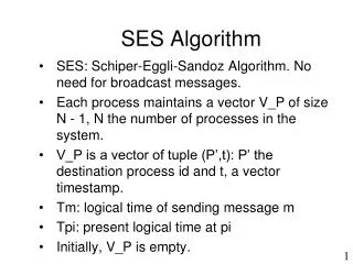
SES Algorithm SES: Schiper-Eggli-Sandoz Algorithm. No need for broadcast messages. Each process maintains a vector V_P of size N - 1, N the number of processes in the system. V_P is a vector of tuple (P’,t): P’ the destination process id and t, a vector timestamp. Tm: logical time of sending message m Tpi: present logical time at pi Initially, V_P is empty. 1
SES Algorithm Sending a Message: Send message M, time stamped tm, along with V_P1 to P2. Insert (P2, tm) into V_P1. Overwrite the previous value of (P2,t), if any. (P2,tm) is not sent. Any future message carrying (P2,tm) in V_P1 cannot be delivered to P2 until tm < tP2. Delivering a message If V_M (in the message) does not contain any pair (P2, t), it can be delivered. /* (P2, t) exists */ If t ≥ Tp2, buffer the message. (Don’t deliver). else (t < Tp2) deliver it 2
SES Algorithm ... What does the condition t ≥ Tp2 imply? t is message vector time stamp. t > Tp2 -> For all j, t[j] > Tp2[j] This implies some events occurred without P2’s knowledge in other processes. So P2 decides to buffer the message. When t < Tp2, message is delivered & Tp2 is updated with the help of V_P2 (after the merge operation). 3
SES Buffering Example (0,0,0) (2,2,2) (1,1,0) Tp1: P1 V_P2: (P1, <0,1,0>) (P3, <0,2,0>) Tp2: (0,1,0) P2 (0,2,0) M1 M2 V_P2: (P1, <0,1,0>) V_P2 empty V_P3: (P1,<0,2,2>) M4 M3 P3 (0,2,1) Tp3: (0,2,2) V_P3: (P1,<0,1,0>) 4
SES Buffering Example... M1 from P2 to P1: M1 + Tm (=<0,1,0>) + Empty V_P2 M2 from P2 to P3: M2 + Tm (<0, 2, 0>) + (P1, <0,1,0>) M3 from P3 to P1: M3 + <0,2,2> + (P1, <0,1,0>) M3 gets buffered because: Tp1 is <0,0,0>, t in (P1, t) is <0,1,0> & so Tp1 < t When M1 is received by P1: Tp1 becomes <1,1,0>, by rules 1 and 2 of vector clock. After updating Tp1, P1 checks buffered M3. Now, Tp1 > t [in (P1, <0,1,0>]. So M3 is delivered. 5
SES Algorithm ... On delivering the message: Merge V_M (in message) with V_P2 as follows. If (P,t) is not there in V_P2, merge. If (P,t) is present in V_P2, t is updated with max(t[i] in Vm, t[i] in V_P2). {Component-wise maximum}. Message cannot be delivered until t in V_M is greater than t in V_P2 Update site P2’s local, logical clock. Check buffered messages after local, logical clock update. 6
SES Algorithm … (1,2,1) (2,2,1) P1 (0,1,1) M2 P2 (0,2,1) V_P2 is empty P3 M1 (0,2,2) (0,0,1) V_P3 is empty 7
Global State Global State 1 C1: Empty $500 $200 C2: Empty A B Global State 2 C1: Tx $50 $450 $200 C2: Empty A B Global State 3 C1: Empty $450 $250 C2: Empty A B 8
Recording Global State... (e.g.,) Global state of A is recorded in (1) and not in (2). State of B, C1, and C2 are recorded in (2) Extra amount of $50 will appear in global state Reason: A’s state recorded before sending message and C1’s state after sending message. Inconsistent global state if n < n’, where n is number of messages sent by A along channel before A’s state was recorded n’ is number of messages sent by A along the channel before channel’s state was recorded. Consistent global state: n = n’ 9
Recording Global State... Similarly, for consistency m = m’ m’: no. of messages received along channel before B’s state recording m: no. of messages received along channel by B before channel’s state was recorded. Also, n’ >= m, as in no system no. of messages sent along the channel be less than that received Hence, n >= m Consistent global state should satisfy the above equation. Consistent global state: Channel state: sequence of messages sent before recording sender’s state, excluding the messages received before receiver’s state was recorded. Only transit messages are recorded in the channel state. 10
Recording Global State Send(Mij): message M sent from Si to Sj rec(Mij): message M received by Sj, from Si time(x): Time of event x LSi: local state at Si send(Mij) is in LSi iff (if and only if) time(send(Mij)) < time(LSi) rec(Mij) is in LSj iff time(rec(Mij)) < time(LSj) transit(LSi, LSj) : set of messages sent/recorded at LSi and NOT received/recorded at LSj 11
Recording Global State … inconsistent(LSi,LSj): set of messages NOT sent/recorded at LSi and received/recorded at LSj Global State, GS: {LS1, LS2,…., LSn} Consistent Global State, GS = {LS1, ..LSn} AND for all i in n, inconsistent(LSi,LSj) is null. Transitless global state, GS = {LS1,…,LSn} AND for all i in n, transit(LSi,LSj) is null. 12
Recording Global State .. LS1 M1 M2 S1 S2 LS2 M1: transit M2: inconsistent 13
Recording Global State... Strongly consistent global state: consistent and transitless, i.e., all send and the corresponding receive events are recorded in all LSi. LS12 LS11 LS22 LS23 LS21 LS33 LS32 LS31 14
Chandy-Lamport Algorithm Distributed algorithm to capture a consistent global state. Communication channels assumed to be FIFO. Uses a marker to initiate the algorithm. Marker sort of dummy message, with no effect on the functions of processes. Sending Marker by P: P records its state. For each outgoing channel C, P sends a marker on C before P sends further messages along C. Receiving Marker by Q: If Q has NOT recorded its state: (a). Record the state of C as an empty sequence. (b) SEND marker (use above rule). Else (Q has recorded state before): Record the state of C as sequence of messages received along C, after Q’s state was recorded and before Q received the marker. FIFO channel condition + markers help in satisfying consistency condition. 15
Chandy-Lamport Algorithm Initiation of marker can be done by any process, with its own unique marker: <process id, sequence number>. Several processes can initiate state recording by sending markers. Concurrent sending of markers allowed. One possible way to collect global state: all processes send the recorded state information to the initiator of marker. Initiator process can sum up the global state. Seq Sj Si Sc Seq’ 16
Chandy-Lamport Algorithm ... Example: Pk Pi Pj Send Marker Send Marker Record channel state Record channel state Record channel state Channel state example: M1 sent to Px at t1, M2 sent to Py at t2, …. 17
Chandy-Lamport Algorithm ... Pi Pj 18
Cuts Cuts: graphical representation of a global state. Cut C = {c1, c2, .., cn}; ci: cut event at Si. Consistent Cut: If every message received by a Si before a cut event, was sent before the cut event at Sender. One can prove: A cut is a consistent cut iff no two cut events are causally related, i.e., !(ci -> cj) and !(cj -> ci). VTc=<3,8 ,6,4> c1 <3,2,5,4> S1 c2<2,7,6,3> S2 <2,8,5,4> c3 S3 c4 S4 19
Time of a Cut C = {c1, c2, .., cn} with vector time stamp VTci. Vector time of the cut, VTc = sup(VTc1, VTc2, .., VTcn). sup is a component-wise maximum, i.e., VTci = max(VTc1[i], VTc2[i], .., VTcn[i]). Now, a cut is consistent iff VTc = (VTc1[1], VTc2[2], .., VTcn[n]). 20
Termination Detection Termination: completion of the sequence of algorithm. (e.g.,) leader election, deadlock detection, deadlock resolution. Use a controlling agent or a monitor process. Initially, all processes are idle. Weight of controlling agent is 1 (0 for others). Start of computation: message from controller to a process. Weight: split into half (0.5 each). Repeat this: any time a process send a computation message to another process, split the weights between the two processes (e.g., 0.25 each for the third time). End of computation: process sends its weight to the controller. Add this weight to that of controller’s. (Sending process’s weight becomes 0). Rule: Sum of W always 1. Termination: When weight of controller becomes 1 again. 21
Huang’s Algorithm B(DW): computation message, DW is the weight. C(DW): control/end of computation message; Rule 1: Before sending B, compute W1, W2 (such that W1 + W2 is W of the process). Send B(W2) to Pi, W = W1. Rule 2: Receiving B(DW) -> W = W + DW, process becomes active. Rule 3: Active to Idle -> send C(DW), W = 0. Rule 4: Receiving C(DW) by controlling agent -> W = W + DW, If W == 1, computation has terminated. 22
Huang’s Algorithm P1 P1 0.5 1/4 P2 P3 P2 P3 0.5 0 1/2 1/16 P4 P5 P4 P5 0 0 1/8 1/16 23