Introduction to Algorithm
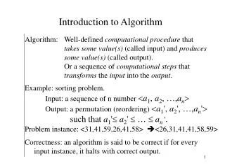
Introduction to Algorithm. Algorithm: . Well-defined computational procedure that takes some value(s) (called input) and produces some value(s) (called output). Or a sequence of computational steps that transforms the input into the output . Example: sorting problem.


Introduction to Algorithm
E N D
Presentation Transcript
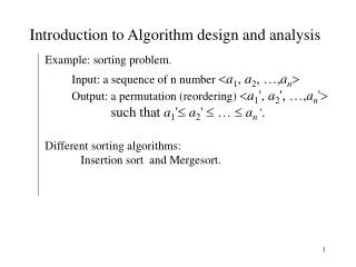
Introduction to Algorithm Algorithm: Well-defined computational procedure that takes some value(s) (called input) and produces some value(s) (called output). Or a sequence of computational steps that transforms the input into the output. Example: sorting problem. Input: a sequence of n number a1, a2, …,an Output: a permutation (reordering) a1', a2', …,an' such that a1' a2' … an '. Problem instance: <31,41,59,26,41,58> <26,31,41,41,58,59> Correctness: an algorithm is said to be correct if for every input instance, it halts with correct output.
Algorithm Design and Analysis • Data structure: the way to store and organize data. • Techniques: • different design and analysis techniques in this course. • purpose is for you to design/analyze your own algorithms for new problems in the future. • Hard problem: • Most problems discussed are efficient (poly time) • An interesting set of hard problems: NP-complete.
NP-complete problem • Why interesting: • Not known whether an efficient algorithm exists for them. • If exist for one, then exist for all. • A small change may cause big change. • Why important: • Arise surprisingly often in real world. • Not waste time on trying to find efficient algorithm to get best solution, instead find approximate or near-optimal solution. • Example: traveling-salesman problem.
Efficiency of Algorithms • Algorithms for solving the same problem can differ dramatically in their efficiency. • much more significant than the differences due to hardware and software. • Comparison of two sorting algorithms (n=106 numbers): • Insertion sort: c1n2 • Merge sort: c2n (lg n) • Best programmer (c1=2), machine language, one billion/second computer. • Bad programmer (c2=50), high-language, ten million/second computer. • 2 (106)2 instructions/109 instructions per second = 2000 seconds. • 50 (106 lg 106) instructions/107 instructions per second 100 seconds. • Thus, merge sort on B is 20 times faster than insertion sort on A! • If sorting ten million number, 2.3 days VS. 20 minutes.
Algorithms as technology • Other modern technologies: • Hardware with high clock rate, pipeline, …. • Easy-to-use, GUI • Object-oriented systems • LAN and WAN • Algorithms are no less important than these. • Moreover, all these new technologies involve heavily algorithms. • More large and complicate problems • As a result, one characteristic separating truly skilled programmer from novices.
Why the course is important • Algorithms as a technology • Suppose computers were infinitely fast and memory was free, is there any need to study algorithm? • Need to find the easiest one to implement. • May be very fast, but not infinitely. • Memory may be very cheap, but not free. • The resources (cpu time and memory) need to be used wisely, (efficient) algorithms will help. • As the basis of computer science discipline. • Core course in computer science/engineering department • (Put emphasis on practical aspects of algorithms).
Insertion Sort Algorithm Input: a sequence of n number a1, a2, …,an Output: a permutation (reordering) a1', a2', …,an' such that a1' a2' … an '. • Idea: (similar to sort a hand of playing cards) • Every time, take one card, and insert the card to correct position in already sorted cards.
Insertion Sort Algorithm (cont.) INSERTION-SORT(A) • forj = 2 to length[A] • dokey A[j] • //insert A[j] to sorted sequence A[1..j-1] • i j-1 • whilei >0and A[i]>key • do A[i+1] A[i] //move A[i] one position right • i i-1 • A[i+1] key
Correctness of Insertion Sort Algorithm • Loop invariant • At the start of each iteration of the for loop, the subarray A[1..j-1] contains original A[1..j-1] but in sorted order. • Proof: • Initialization : j=2, A[1..j-1]=A[1..1]=A[1], sorted. • Maintenance: each iteration maintains loop invariant. • Termination: j=n+1, so A[1..j-1]=A[1..n] in sorted order. • Pseudocode conventions
Analyzing algorithms • Time (not memory, bandwidth, hardware) • Implementation model • Random-Access-Model (RAM) • One processor, sequential execution, no concurrency. • Basic data types • Basic operations (constant time per operation) • (Parallel multi-processor access model: PRAM)
Analysis of Insertion Sort INSERTION-SORT(A) costtimes • forj = 2 to length[A] c1n • dokey A[j] c2n-1 • //insert A[j] to sorted sequence A[1..j-1] 0n-1 • i j-1 c4n-1 • whilei >0and A[i]>keyc5j=2n tj • do A[i+1] A[i] c6j=2n(tj –1) • i i-1 c7j=2n(tj –1) • A[i+1] key c8n–1 (tj is the number of times the while loop test in line 5 is executed for that value of j) The total time cost T(n) = sum of cost times in each line =c1n + c2(n-1) + c4(n-1) + c5j=2n tj+ c6j=2n (tj-1)+ c7j=2n (tj-1)+ c8(n-1)
Analysis of Insertion Sort (cont.) • Best case cost: already ordered numbers • tj=1, and line 6 and 7 will be executed 0 times • T(n) = c1n + c2(n-1) + c4(n-1) + c5(n-1) + c8(n-1) =(c1 + c2 + c4 + c5 + c8)n – (c2 + c4 + c5 + c8) = cn + c‘ • Worst case cost: reverse ordered numbers • tj=j, • so j=2n tj = j=2n j =n(n+1)/2-1, and j=2n(tj –1) = j=2n(j–1) = n(n-1)/2, and • T(n) = c1n + c2(n-1) + c4(n-1) + c5(n(n+1)/2 -1) + + c6(n(n-1)/2 -1) + c7(n(n-1)/2)+ c8(n-1) =((c5 + c6 + c7)/2)n2 +(c1 + c2 + c4 +c5/2-c6/2-c7/2+c8)n-(c2 + c4 + c5 + c8) =an2+bn+c • Average case cost: random numbers • in average, tj = j/2. T(n) will still be in the order of n2, same as worst case.
The Worst Case Running Time • An upper bound for any input. • For some algorithms, worst case occurs often. • Average case is often roughly as bad as the worst case.
Order of growth • Lower order item(s) are ignored, just keep the highest order item. • The constant coefficient(s) are ignored. • The rate of growth, or the order of growth, possesses the highest significance. • Use (n2) to represent the worst case running time for insertion sort. • (1), (lg n), (n),(n), (nlg n), (n2), (n3), (2n), (n!)
Design Approaches • Recursive algorithm • To solve a given problem, the algorithm recursively calls itself one or more time to deal with closely related subproblems. • f(n) = 0 if n=1 1 if n=2 f(n-1) + f(n-2), if n>2 • Divide-and-conquer • Dynamic programming • Prune-and-search • Greedy algorithms, Linear programming, Parallel algorithms, Approximate algorithms, etc.
Divide-and-conquer approach • Divide the problem into a number of subproblems, with the same type as the original problem type. • Conquer the subproblems by solving them recursively. If the size of a subproblem is small enough, just solve the subproblem directly. • Combine the solutions to the subproblems into the solution for the original problem.
Merge Sort • Divide: divide the n-element sequence into two subproblems of n/2 elements each. • Conquer: sort the two subsequences recursively using merge sort. If the length of a sequence is 1, do nothing since it is already in order. • Combine: merge the two sorted subsequences to produce the sorted answer.
Merge Sort –merge function • Merge is the key operation in merge sort. • Suppose the (sub)sequence(s) are stored in the array A. moreover, A[p..q] and A[q+1..r] are two sorted subsequences. • MERGE(A,p,q,r) will merge the two subsequences into sorted sequence A[p..r]
MERGE(A,p,q,r) • n1 q – p + 1 • n2 r – q • //createtemporaryL[1..n1+1], R[1..n2+1] • fori 1 ton1 • do L[i] A[p+i-1] • forj 1 ton2 • do R[j] A[q+j] • L[n1 +1] • R[n2 +1] • i 1 • j 1 • Fork ptor • do if L[i] R[j] • then A[k] L[i] • i i+1 • else A[k] R[j] • j j+1
Correctness of MERGE(A,p,q,r) • Loop invariant • At start of each iteration of for loop of line 12-17, subarray A[p..k-1] contains the k-p smallest elements of L[1..n1+1] and R[1..n2+1] in sorted order. L[i] and R[j] are smallest elements of their arrays that have not been copied back to A. • Proof: • Initialization: k-p=0, i=j=1, L[1] and R[1] are smallest. • Maintenance: loop will maintain the invariant • Termination: k=r+1, so A[p..k-1]= A[p..r] contains all and in sorted.
Analysis of MERGE(A,p,q,r) • n1 q – p + 1 (1) • n2 r – q (1) • //createtemporaryL[1..n1+1], R[1..n2+1] (0) • fori 1 ton1 (n1) (n1 +1 times) • do L[i] A[p+i-1] (1)* (n1) (n1 times) • forj 1 ton2 (n2) (n2 +1 times) • do R[j] A[q+j] (1) * (n2) (n2 times) • L[n1 +1] (1) • R[n2 +1] (1) • i 1 (1) • j 1 (1) • Fork ptor (n), suppose n = r-p+1 • do if L[i] R[j] (1)*(n) • then A[k] L[i] (1)*O(n) • i i+1 (1)*O(n) • else A[k] R[j] (1)*O(n) • j j+1 (1)*O(n) Thus the total running time is (n1)+ (n2)+ (n)+7 (1) = (n).
MERGE-SORT(A,p,r) • ifp < r • thenq (p+r)/2 • MERGE-SORT(A,p,q) • MERGE-SORT(A,q+1,r) • MERGE(A,p,q,r) Call to MERGE-SORT(A,1,n) (suppose n=length(A))
Analysis of Divide-and-Conquer • Described by recursive equation • Suppose T(n) is the running time on a problem of size n. • T(n) = (1) if nc aT(n/b)+D(n)+C(n) if n>c Where a: number of subproblems n/b: size of each subproblem D(n): cost of divide operation C(n): cost of combination operation
Analysis of MERGE-SORT • Divide: D(n) = (1) • Conquer: a=2,b=2, so 2T(n/2) • Combine: C(n) = (n) • T(n) = (1) if n=1 2T(n/2)+ (n) if n>1 • T(n) = c if n=1 2T(n/2)+ cn if n>1
Compute T(n) by Recursive Tree • The recursive equation can be solved by recursive tree. • T(n) = 2T(n/2)+ cn, (See its Recursive Tree). • lg n+1 levels, cn at each level, thus • Total cost for merge sort is • T(n) =cnlg n +cn = (nlg n). • In contrast, insertion sort is • T(n) = (n2).
Growth of functions • Asymptotic efficiency: • Input size is very large • Ignore lower-order terms and constant coefficients • Only the highest order item, (order of growth). • Typical order of growth: • (1), (lg n), (n),(n), (nlg n), (n2), (n3), (2n), (n!) • Asymptotic notations: O, , , o, .
-notation • For a given function g(n), • (g(n))={f(n): there exist positive constants c1,c2,and n0 such that 0 c1g(n) f(n) c2g(n) for all n n0} • Write f(n) (g(n)), or simply f(n) = (g(n)). c2g(n) f(n) c1g(n) n n0 f(n) = (g(n))
Some (g(n)) functions • Prove 1/2n2 – 3n = (n2). • c1 n2 1/2n2 – 3n c2 n2 • c1 1/2 – 3/n c2 • c2 ½ for any n 1, and c1 1/14 for any n 7 • Thus, c1= 1/14, c2 = ½ , n0=7. • Prove 6n3 (n2). • In general, f(n)=an2+bn+c = (n2), where a,b,c are constants and a>0. • p(n) = i=0daini, where ai are constants and ad>0. • then p(n) = (nd). • (n0) or (1), constant time complexity.
O-notation • For a given function g(n), • O(g(n))={f(n): there exist positive constants c and n0 such that 0 f(n) cg(n) for all n n0} • Write f(n) O(g(n)), or simply f(n) = O(g(n)). cg(n) f(n) n n0 f(n) = O(g(n))
Relation between (g(n)) and O(g(n)) • f(n) = (g(n)) implies f(n) = O(g(n)) • -notation is a stronger notion than O-notation. • (g(n)) O(g(n)) • an2+bn+c = (n2), also =O(n2) • A little surprising: an+b = O(n2). Verify it!!! • Even n =O(n2) !!! • O-notation, represents asymptotic upper bound. • -notation, represents asymptotic tight bound. • Note for distinctions: • When we say worst-case running time for insertion sort is O(n2), which applies to all inputs, even an already sorted input runs only in O(n) time because O(n) O(n2). • However, worst-case running time (n2) for insertion sort does not apply to every input, since for an already sorted input, (n) (n2) .
-notation • For a given function g(n), • (g(n))={f(n): there exist positive constants c and n0 such that 0 cg(n) f(n) for all n n0} • Write f(n) (g(n)), or simply f(n) = (g(n)). f(n) cg(n) n n0 f(n) = (g(n))
Relation among O, ,-notations • Theorem 3.1 (page 46) • For f(n) and g(n), f(n) = (g(n)) if and only if f(n) = O(g(n)) and f(n) = (g(n)). • O-notation: asymptotic upper bound. • -notation: asymptotic tight bound. • -notation: asymptotic lower bound.
Notes on -notation • generally used for best case running time. • So correct for all inputs. • For example, in insertion sort • best case running time is (n), • or correctly say: running time is (n). • It is OK to say worst case running time is (n2) • However, it is incorrect to say running time is (n2).
o-notation • For a given function g(n), • o(g(n))={f(n): for any positive constant c,there exist a positive n0 such that 0 f(n) cg(n) for all n n0} • Write f(n) o(g(n)), or simply f(n) = o(g(n)). 2g(n) g(n) 1/2g(n) f(n) n n0 n0 n0 f(n) = o(g(n))
g(n) n Notes on o-notition • O-notation may or may not be asymptotically tight for upper bound. • 2n2 = O(n2) is tight, but 2n = O(n2) is not tight. • o-notition is used to denote an upper bound that is not asymptotically tight. • 2n = o(n2), but 2n2o(n2). • Difference: for some positive constant c in O-notation, but all positive constants c in o-notation. • In o-notation, f(n) becomes insignificant relative to g(n) as n approaches infinitely: i.e., • lim = 0. f(n)
-notation • For a given function g(n), • (g(n))={f(n): for any positive constant c, there exists a positive n0 such that 0 cg(n) f(n) for all n n0} • Write f(n) (g(n)), or simply f(n) = (g(n)). • -notation, similar to o-notation, denotes lower bound that is not asymptotically tight. • n2/2 = (n), but n2/2 (n2) • f(n) = (g(n)) if and only if g(n)=o(f(n)). • lim = f(n) g(n) n
Properties of asymptotic notations • Transitivity: all five notations • f(n)= (g(n)) and g(n)= (h(n)) f(n)= (h(n)) • Reflexivity: O, , notations. • f(n)= (f(n)) • Symmetry: notation. • f(n)= (g(n)) if and only if g(n)= (f(n)) • Transpose symmetry: • f(n) = O(g(n)) if and only if g(n)= (f(n)). • f(n) = o(g(n)) if and only if g(n)= (f(n)).
Asymptotic Efficiency of Recurrences • Find the asymptotic bounds of recursive equations. • Substitution method • Recursive tree method • Master method (master theorem) • Provides bounds for: T(n) = aT(n/b)+f(n) where • a 1 (the number of subproblems). • b>1, (n/b is the size of each subproblem). • f(n) is a given function.
Recurrences • MERGE-SORT • T(n) = (1) if n=1 2T(n/2)+ (n) if n>1 • Ignore certain details: • T(n) = (1) if n=1 T(n/2)+ T(n/2)+ (n) if n>1 • Moreover, T(n) = 2T(n/2)+ (n)
The Substitution Method • Two steps: • Guess the form of the solution. • By experience, and creativity. • By Some heuristics. • If a recurrence is similar to one you have seen before. • T(n)=2T(n/2+17)+n, similar to T(n)=2T(n/2)+n, , guess O(nlg n). • Prove loose upper and lower bounds on the recurrence and then reduce the range of uncertainty. • For T(n)=2T(n/2)+n, prove lower bound T(n)= (n), and prove upper bound T(n)= O(n2), then guess the tight bound is T(n)=O(nlg n). • By recursion tree. • Use mathematical induction to find the constants and show that the solution works.
Solve T(n)=2T(n/2)+n • Guess the solution: T(n)=O(nlg n), • i.e., T(n)cnlg n for some c. • Prove the solution by induction: • Suppose this bound holds for n/2, i.e., • T(n/2)cn/2lg (n/2). • T(n) 2(cn/2lg (n/2))+n • cnlg (n/2))+n • = cnlg n - cnlg 2 +n • = cnlg n - cn +n • cnlg n (as long as c1) • Is the above proof complete? Why?
Boundary (base) Condition • In fact, T(n) =1 if n=1, i.e., T(1)=1. • However, cnlg n =c1lg 1 = 0, which is odd with T(1)=1. • Take advantage of asymptotic notation: it is required T(n)cnlg n hold for n n0 where n0 is a constant of our choosing. • Select n0 =2, thus, n=2 and n=3 as our induction bases. It turns out any c 2 suffices for base cases of n=2 and n=3 to hold.
Subtleties • Guess is correct, but induction proof not work. • Problem is that inductive assumption not strong enough. • Solution: revise the guess by subtracting a lower-order term. • Example: T(n)=T(n/2)+T(n/2)+1. • Guess T(n)=O(n), i.e., T(n) cn for some c. • However, T(n) c n/2+c n/2+1 =cn+1, which does not imply T(n) cn for any c. • Attempting T(n)=O(n2) will work, but overkill. • New guess T(n) cn – b will work as long as b 1.
Avoiding Pitfall • It is easy to guess T(n)=O(n) (i.e., T(n) cn) for T(n)=2T(n/2)+n. • And wrongly prove: • T(n) 2(cn/2)+n • cn+n • =O(n). wrongly !!!! • Problem is that it does not prove the exactform of T(n) cn.