A New Linear Algorithm for Checking Graph 3-Edge-Connectivity

1. A new linear algorithm for checking a graph for 3-edge-connectivity Feng Sun Advisor: Dr. Robert W. Robinson Committee: Dr. E. Rodney Canfield Dr. Eileen T. Kraemer 2003.2

2. Outline • Overview • Concepts and definitions • Analysis of separation pairs • Test results

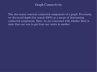
3. Graph Connectivity • Applications • Network reliability • Planar graph • Vertex Connectivity (κ) • Edge Connectivity (λ) • Our algorithm • Check whether a graph is 3-edge-connected in O(m+n) time • Based on Depth-first search • Modified from the algorithm of Hopcroft and Tarjan to divide a graph into 3-vertex-connected components

4. An example of a 3-edge-connnected graph

5. Concepts • Graph • An ordered pair of disjoint sets (V, E), where V is the vertex set and E is the edge set. E is a subset of the set V(2)of unordered pairs from V. • The order of a graph is |V| and the size of a graph is |E|. • A graph is labeled if the integers from 1 through n are assigned to its vertices. An unlabeled graph is an isomorphism class of labeled graphs. • Tree • Acyclic connected graph • A subgraph which contains all the vertices of a graph is the spanning tree of the graph • Edge separator • A minimal edge set S such that removal of S from a graph G disconnect G. • A graph is k-edge-connected if every edge-separator has at least k edges. • The edge connectivity of a graph G of order n ≥ 2 is the minimum cardinality of an edge-separator.

6. Concepts (cont.) • Palm tree • Let P be a directed graph consisting of two disjoint sets of edges denoted by v→w and v --→w. P is a palm tree if P satisfies the following properties: • The subgraph T containing the edges v→w is a spanning tree of P. • If v --→w, then w*→v. That is, each edge not in the spanning tree of P connects a vertex with one of its ancestors in T. The edges v --→w are called the fronds of P. 1 2 3 4

7. Depth-first Search ALGORITHM DFS(G) 1 FOR each vertex v in V(G) 2 NUMBER(v) = FATHER(v) = 0; 3 time = 0; 4 DFS-VISIT(root); END ALGORITHM PROCEDURE DFS-VISIT(v) 1 NUMBER(v) = time = time + 1 2 FOR w in the adjacency list of v DO 3 { 4 IF NUMBER(w) == 0 THEN 5 { 6 mark vw as a tree edge in P; 7 FATHER(w) = v; 8 DFS-VISIT(w); 9 } 10 ELSE IF NUMBER(w) < NUMBER(v) and w != FATHER(v) THEN 11 mark vw as a frond in P; 12 }

8. Identifying separation pairs • Three cases if a graph G is not 3-edge-connected • Not connected • Connected but not 2-edge-connected • 2-edge-connected but not 3-edge-connected • Separation pair

9. a w u t v G1 G1 d x v (a) Type 1 (b) Type 2 Two types of separation pairs in a palm tree • Type 1: One tree edge, one frond • Type 2: Two tree edges

10. Important values for identifying type 1 pair

11. An Expanded DFS PROCEDURE FIRSTDFS-VISIT(v) 1 NUMBER(v) = time = time + 1; 2 LOWPT1(v) = LOWPT2(v) = NUMBER(v); 3 ND(v) = 1; 4 FOR w in the adjacency list of v DO 5 { 6 IF NUMBER(w) == 0 THEN 7 { 8 mark vw as a tree edge in P; 9 FATHER(w) = v; 10 FIRSTDFS-VISIT(w); 10.1 IF ( LOWPT1(w) < v and LOWPT2(w) >= w ) THEN 10.2 detect a type 1 separation pair, procedure stop; 11 IF LOWPT1(w) < LOWPT1(v) THEN 12 { 13 LOWPT2(v) = MIN{LOWPT1(v), LOWPT2(w)}; 14 LOWPT1(v) = LOWPT1(w); 15 } 16 ELSE IF LOWPT1(w) == LOWPT1(v) THEN 17 LOWPT2(v) = LOWPT1(w); 18 ELSE 19 LOWPT2(v) = MIN{LOWPT2(v), LOWPT1(w)}; 20 ND(v) = ND(v) + ND(w); 21 } 22 ELSE IF NUMBER(w) < NUMBER(v) and w != FATHER(v) THEN 23 { 24 mark vw as a frond in P; 25 IF NUMBER(w) < LOWPT1(v) THEN 26 { 27 LOWPT2(v) = LOWPT1(v); 28 LOWPT1(v) = NUMBER(w); 29 } 30 ELSE IF NUMBER(w) == LOWPT1(v) THEN 31 LOWPT2(v) = NUMBER(w); 32 ELSE 33 LOWPT2(v) = MIN{LOWPT2(v), NUMBER(w)}; 34 } 35 }

12. a LOWPT1(w) u w x LOWPT2(w) ≥ w Identify type 1 separation pair

13. Preparation steps for type 2 pair

14. Decrease A(1) A(1) B(2) Decrease B(2) F(6) F(6) C(3) C(3) G(7) H(8) H(8) G(7) E(4) Preparation Steps for type 2 pair (cont.) (ii) After D(5) D(4) E(5) (i) Before

15. Properties of the palm tree

16. Identify type 2 separation pair 1 u a y1 2 v x1 y2 b 3 x2

17. Step to identify type 2 pair

18. The DFS to identify type 2 pair PROCEDURE PATHSEARCH-DFS(v) (input: vertex v is the current vertex in the depth-first search) 1 FOR w IN A(v) DO 2 { 3 IF vw is a tree edge THEN 4 { 5 IF vw is a first edge of a path THEN 6 { 7 IF LOWPT1(w) < LOWEST(v) and w is not A1(v) THEN 8 LOWEST(v) = LOWPT1(w); 9 add end-of-stack marker to PStack; 10 } 11 returnVal = PATHSEARCH-DFS(w); 12 IF returnVal == 0 THEN 13 return 0; 14 } 15 ELSE // vw is a frond 16 IF NUMBER(w) < LOWEST(v) THEN 17 LOWEST(v) = NUMBER(w); 18 } 19 WHILE (a, b) on PStack satisfies a <= NUMBER(v) < b and LOWEST(v) < a 20 remove (a, b) from PStack; 21 IF no pair deleted from PStack THEN 22 add ( LOWEST(v), A1(v) ) to PStack; 23 IF (a, b) is the last pair deleted from PStack THEN 24 add ( LOWEST(v), b ) to PStack; 25 WHILE (a, b) on PStack satisfies a <= NUMBER(v) < b and HIGHPT(v) >= b 26 remove (a, b) from PStack; 27 WHILE (a, b) on PStack satisfies a = v 28 { 29 IF ( b <= a or a == 0 ) THEN 30 delete (a, b) from PStack; 31 ELSE //we find type 2 pair {(FATHER(a), a), (FATHER(b), b)} 32 return 0; 33 } 34 IF ( FATHER(v), v) is a first edge of a path THEN 35 delete all entries on PStack down to and including end-of-stack marker; 36 return 1;

19. parent(LOWEST(v)) a’ LOWEST(v) a a v v b w b w x highpt(v) Cases for lines 20 and 26 If LOWEST(v) < a, (parent(LOWPT1(w)), LOWPT1(w)) and (parent(b), b) become the new potential separation pair. We use (b, lowest(v) ) to substitute (b, a) in the PStack. If hightpt(v) >= b, (a, b) will be deleted from PStack.

20. 0 2 3 4 1 Implementation and Test Results • General graph • Check graphs generated by Nauty • Numbers of labeled and unlabeled 3-edge-connected graphs up to order 11. • Numbers of labeled and unlabeled 3-edge-connected blocks up to order 11. • The above numbers for labeled graphs and for unlabeled 3-edge-connected blocks were provided by S. K. Pootheri. • Compare with Z. Chen’s algorithm for higher order random graphs • Feynman diagrams • Compare with Qun Wang’s quadratic algorithm 5

21. Numbers of unlabeled and labeled 3-edge-connected graphs by order n

22. Numbers of unlabeled 3-edge-connected graphs by order n and size m

23. Average testing times and scaled times for two algorithms on random graphs • For each 100 random graphs were generated and about half of them are 3-edge-connected • The scaled time is the actual testing time divided by m+n

24. Comparison of running times and scaled times for 3-edge-connectivity

25. Comparison of running times for our linear algorithm and a quadratic algorithm on Feynman diagrams • Use a simplified algorithm for Feynman diagram • Feynman diagrams were generated by a program wrote by Dr. Robinson • Q. Wang developed three algorithm for testing 3-edge-connectivity of a Feynman diagram. The quadratic algorithm is the best for order less than 12

26. Conclusions and future work • A new linear algorithm for determining whether a graph is 3-edge-connected is presented. • A variation of the algorithm was developed specifically for testing Feynman diagrams. • Tests showed that the implementations are correct and also faster than the available alternatives. • A promising future direction is to extend our algorithm to deal with fully dynamic 3-edge-connectivity problem.

27. Acknowledgements • Dr. Robert W. Robinson • Dr. E. Rodney Canfield • Dr. Eileen T. Kraemer • Dr. David K. Lowenthal • Other professors, staffs and students in our department