Estimating Exchange Rates in Tidal Estuaries Using ROMS and Lagrangian Float Simulations
This research explores the use of ROMS and Lagrangian float simulations to estimate exchange rates between spatial compartments in a tidal estuary. Our primary aim is to ascertain the maximum carrying capacity of a selected bay for mussel aquaculture. By coupling a fine-resolution hydrodynamic model with a coarse-resolution transport model, we calculate exchange rates through tracer observations. Initial findings indicate that Lagrangian float calculations outperform naive methods for evaluating transfer coefficients, effectively addressing inaccuracies stemming from sharp initial field edges.

Estimating Exchange Rates in Tidal Estuaries Using ROMS and Lagrangian Float Simulations
E N D
Presentation Transcript
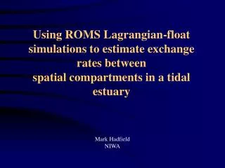
Using ROMS Lagrangian-float simulations to estimate exchange rates betweenspatial compartments in a tidal estuary Mark HadfieldNIWA
Outline • Research strategy • Setting • Box modelling • POL3D and Eulerian tracers • ROMS and Lagrangian floats • Preliminary results • Conclusions
Strategy • We want to estimate maximum carrying capacity of a selected bay for mussel aquaculture. • Couple a fine-resolution hydrodynamic model with a coarse resolution transport/ecology model (a “spatially aggregated” or “box” model). • Coupling achieved by having the hydrodynamic model calculate exchange rates between the boxes. • Exchange rates to be estimated in the hydrodynamic model using tracers: label each box with a tracer and observing the rate of exchange with other boxes.
Box Model Formulation Fij = TijCi Ci Cj Fji = TjiCj Fij – Fji = TijCi –TjiCj = TD(Ci – Cj) + TA(Ci + Cj) / 2 where TD = (Tij + Tji) / 2 TA = Tij + Tji
Evaluating coefficients:the naïve approach At a specified time, label each box with a separate tracer with concentration = 1. After a suitable interval Dt measure the mass Mij of each tracer i in every other box j. Then Tij » Mij/ Dt.
Earlier Simulations —POL3D, Eulerian tracer • Proudman Oceanographic Laboratory 3D model (POL3D) • Grid covering Pelorus Sound, 141 140 points, 18 levels, horizontal spacing 250 m. • Forced at outer boundary by M2 tide (amplitude 0.88 m). • Two-day flood event beginning at 3 days • Rainfall on surface of sound, then Pelorus River flow peak. • After the flood, river flow and rainfall continue at lower rates • Eulerian tracers released and followed for 5 tidal cycles
Current Simulations –ROMS, Lagrangian tracer • ROMS • Rectangular grid, 250 m horizontal spacing, 15 levels with moderate vertical stretching. • Large, McWilliams, Doney (LMD) vertical mixing. • Forcing as before. • Float trajectories deterministic for now, i.e. no random walk.
Exchange calculations • 500, 000 Lagrangian floats, initially distributed uniformly throughout the domain, released and tracked for 5 tidal cycles. • At any instant we can mark out a region in the fluid, label the particles in that region, then follow them for the remainder of the float simulation. • The results of several such pseudo-releases are averaged to eliminate: • variations with tidal phase • stochastic effects
Conclusions • The naïve method of evaluating transfer coefficients from tracer exchange data has problems due to sharp edges in the initial fields • With Lagrangian float calculations we can use the extra trajectory information to solve those problems.