Radiation schemes in a NWP or climate GCM
440 likes | 660 Vues
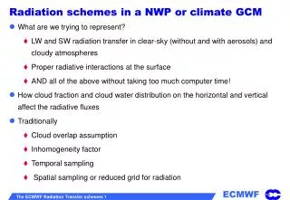
Radiation schemes in a NWP or climate GCM. What are we trying to represent? LW and SW radiation transfer in clear-sky (without and with aerosols) and cloudy atmospheres Proper radiative interactions at the surface AND all of the above without taking too much computer time!

Radiation schemes in a NWP or climate GCM
E N D
Presentation Transcript
Radiation schemes in a NWP or climate GCM • What are we trying to represent? • LW and SW radiation transfer in clear-sky (without and with aerosols) and cloudy atmospheres • Proper radiative interactions at the surface • AND all of the above without taking too much computer time! • How cloud fraction and cloud water distribution on the horizontal and vertical affect the radiative fluxes • Traditionally • Cloud overlap assumption • Inhomogeneity factor • Temporal sampling • Spatial sampling or reduced grid for radiation
Role of the cloud overlap assumption - 1 (Morcrette and Jakob, 2000: Mon.Wea.Rev., 128, 1707-1732) • Part of the inhomogeneity seen from satellite measurements of optical thickness is linked to the vertical piling up of cloud layers. • In GCMs, various cloud overlap assumptions can be used, among them:
The inhomogeneity problem • “Inhomogeneities” in the spatial distribution of the cloud water arise because of: • sub-grid variations unaccounted for in the one profile / grid box approach • cloud overlapping in the vertical • the spatial (and temporal) sampling in the full radiation computations
Impact of sub-grid distribution of cloud water - 1 • Work by Cahalan, Barker and others have shown that inhomogeneities in the spatial distribution of cloud water are likely to affect the radiation transfer within clouds.
On the effect of the spatial (and temporal) sampling of radiation calculations (Morcrette, 2000, Mon.Wea.Rev., 128, 876-887) • In the pre-2002 operational model, full radiation was computed every 3 hours (every 1 hour during the 12-hour first-guess forecast used for analysis), and on a reduced spatial grid, with only 1 point out of 4 in the tropics. • What is the impact of such strategy for economy of computer time? Impact on anomaly correlation of geopotential is negligible
Not surprisingly • the cloud overlap assumption, • an inhomogeneity treatment, if introduced, • any spatial and/or temporal sampling has some impact, sometimes large, on the 4D-distribution of radiative heating rate, temperature, humidity and cloud cover and cloud water distributions in the atmosphere.
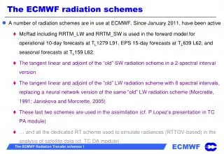
The ECMWF radiation schemes: present and future • Before cycle32r3 and, concerning LW, since cycle22r3 – includes ERA-40 and ERA-Interim • SW following a photon path distribution method originally from Fouquart and Bonnel (1980). [see lecture notes for details] • LW: the Rapid Radiation Transfer Model (Mlawer et al., 1997) • Since cycle32r3 replaced by by McRAD • LW: as above • SW: using the RRTM approach, consistent spectroscopic database and absorption coefficients • Using the McICA (Monte-Carlo Independent Column Approximation) to deal with radiation transfer in cloudy atmospheres
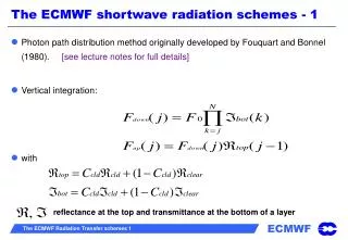
The ECMWF shortwave radiation schemes - 1 • Photon path distribution method originally developed by Fouquart and Bonnel (1980). [see lecture notes for full details] • Vertical integration: • with reflectance at the top and transmittance at the bottom of a layer
The ECMWF shortwave radiation schemes - 2 • Delta-Eddington method (Shettle and Weinman, 1970; Joseph et al., 1976) to compute from the total optical thickness , single scattering albedo , and asymmetry factor g, which account for the combined effect of cloud condensed water, aerosol, and molecular absorption
The ECMWF shortwave radiation schemes - 2 • Laplace transform method to get the photon path equivalent gaseous absorber amounts from 2 sets of layer reflectances and transmittances, assuming successively a non-reflecting underlying medium ( ) then a reflecting one ( ) • where are the layer reflectance and transmittance corresponding to a conservative scattering medium and ke is an absorption coefficient approximating the spectrally averaged transmission of the clear-sky atmosphere
The ECMWF shortwave radiation schemes - 3 • Transmission functions for O3, H2O, CO2, N2O, CH4 are fitted with Pade approximants from reference calculations
SW6 vs. SW4 • 6 spectral intervals from 0.185 to 4 mm • Based on a line-by-line model of the transmission functions • LbL based on STRANSAC (Scott, 1974, Dubuisson et al., 1996) • modified to account for HITRAN 2000 • H2O, CO2, O3, O2, CH4, CO, N2O • resolution 0.01 cm-1 from 2000 to 20000 cm-1, then resolution of the O3 continuum, i.e. 5 to 10 cm-1 • UVCBA in 2 intervals, 0.185-0.25-0.4 mm, visible in 1 interval, 0.4-0.69 mm 4 spectral intervals from 0.25 to 4 mm Based on statistical models of the transmission functions UVBA and visible in one interval from 0.25 to 0.69 mm
The SW_6 radiation scheme - 2 Comparison with a line-by-line model of the SW radiation transfer on standard cases shows an excellent agreement on the flux profiles surface Standard tropical atmosphere: full line = LbL dash line = SW6 Top of the atmosphere
RRTM vs. M91/G00 - 1 The ECMWF LW radiation schemes: RRTM_LW vs. M91/G00 00
M91/G00 Morcrette, 1991, JGR, 96D, 9121-9132 Gregory et al., 2000, QJRMS, 126A, 1685-1710. • Band-emissivity type of scheme, i.e., solves for a (N+1)2 matrix of transmission functions • Six spectral intervals • 0-350 + 1450-1680 cm-1 970-1110 cm-1 • 500-800 cm-1 350-500 cm-1 • 800-970 cm-1 1250-1450 + 1880-2820 cm-1 • mixed vertical quadrature: • 2-point Gaussian for layers adjacent to level of computation • trapezoidal rule for distant layers
M91/G00 - 2 • Transmission functions represented by Pade approximants from transmission functions computed with Malkmus and Goody statistical models • with the effective absorber amount Diffusivity factor Pressure-weighted amount of absorber
M91/G00 - 3 • Effective cloudiness • kabs,liq from Smith and Shi (1992), kabs,ice from Ebert and Curry (1992) • Effect of clouds on LW fluxes following Washington and Williamson (1977). Formulation allows for maximum, maximum-random, or random cloud overlap.
RRTM_LW Mlawer et al., 1997: JGR, 102D, 16663-16682 Morcrette et al., 1998: ECMWF Tech.Memo., 252 • The use of the correlated-k method (mapping k -> g) allows radiative transfer to be performed as a monochromatic process Ro is the radiance incoming to the layer, B(n,T) the Planck function at wavenumber n and temperature T tn is the transmittance for the layer optical path t’n the transmittance at a point along the layer optical path Discretized over j (k, k+Dk) intervals of width Wj
RRTM_LW vs. M91/G00 - 1 MLS profile
RRTM_LW vs. M91/G00 - 2 Morcrette et al., 2001, ECMWF Newsletter, 91, 2-9. • Due to the increased LW absorption, RRTM provides smaller OLR and larger surface downward LW radiation For clear-sky situations For overcast low- and high-level cloudiness
RRTM vs. M91/G00 - 3 Differences in OLR: RRTM-M91/G00 OLR derived from AVHRR from April 99 OLR from ECMWF model with RRTM
Recent developments: to become operational in May 2007 • A new set of radiation parametrisations has recently been developed. Each component has been tested independently, then together. • It includes a replacement of the spectrally flat ERBE-derived land surface albedo by a multi-component albedo derived from MODIS observations • It also replace the SW scheme by a RRTM-based SW scheme • Clouds are treated using the McICA approach • This set has been extensively tested in pre-operational mode and will become operational in May 2007
MODIS Albedo • Replace the climatology of spectrally flat land albedo derived from ERBE by a new climatology of UVis, Near-IR albedos for direct and diffuse components derived from 4 years (2001-2004) of MODIS data. • Available at all TL resolutions from 95 to 1279 • At present, only the snow-free land surface albedo is changed. No albedo changes to snow, sea-ice, Greenland or Antarctica. A sensitivity study on the role of snow and sea-ice albedo would be interesting and is to be conducted. • Small impact in FCs
What is McICA? It is an attempt at dealing with the following question: How to best represent the radiative effect of clouds knowing that they are vertical and horizontal sub-grid scale entities with variability in cloud liquid, mixed-phase and ice water?
A bit of vocabulary and some references • CKD: Correlated k-distribution • ICA: Independent Column Approximation • McICA: Monte-Carlo Independent Column Approximation • PPH: Plane Parallel Homogeneous • RT: Radiative Transfer • A full description of the McICA approach with details on the cloud generators and other computational aspects can be found in the following publications: • Barker et al., 2003: GCSS/ARM Workshop, Kananaskis, Alb • Pincus et al., 2003: JGR, 108D, 4376 • Barker, Raisanen, 2004: QJRMS 130,1905-1920 • Raisanen et al., 2004: QJRMS 130, 2047-2067 • Raisanen, Barker, 2004: QJRMS 130, 2069-2085 • Barker, Raisanen, 2005: QJRMS 131, 3103-3122 • Raisanen et al., 2005: J. Climate 18, 4715-4730.
What is McICA? • Monte-Carlo Independent Column Approximation • The CKD approach for 1-D PPH columns is • The ICA approach for domain averages is (ICA: Independent Column Approx.) • Combining (1) and (2) gives • Assuming clear- and cloudy-sky columns of gas, and if there are Nc cloudy columns, (3) can be written as Correlated-k distributed absorption coefficients as in RRTM (1) (2) (3)
What is McICA? • Which can be simplified to • The hypothesis is that can be given by • In which case, it follows (see Barker’s May 2002 presentation) that The model is unbiased in the ICA sense, so for T=K * Nc large enough, an unbiased value can be obtained using a different random cloud profile for each k-coefficient
The ECMWF McRad configuration = RRTM_LW + RRTM_SW + McICA + cloud optical properties • RRTM_SW from AER, Inc, with reduced number of g-points from the original 224 to 112 • RRTM_SW is more expensive than SW6 (see later) • McICA version for both RRTM_LW and RRTM_SW: no cloud fraction anymore: a layer is either clear-sky or overcast • McICA does not cost anything (as such) • Random generator (Raisanen et al, 2004) gives 0 or 1 cloud for each layer and each of the 140 (112) g-points of the LW (SW) radiation scheme for either a maximum-random or a generalized overlap assumption, with loose constraint over the total cloudiness • “New” cloud optical properties (main point: De=f(IWC,T)) • In the following, results are shown for the generalized overlap (a la Hogan and Illingworth, 2000) with a decorrelation length of 2km for cloud fraction, and 1km for cloud condensate (see later)
McRad: A state of the art method for representing cloud-radiation interactions in the ECMWF model • McICA allows a consistent approach on the definition of cloud overlap not only between LW and SW radiation, but also with other physical processes (precipitation/evaporation) (Jakob and Klein, 1999, 2000). • RRTM_SW with 112 g-points is a “good scheme” to get the full benefit of McICA. It improves the temperature in the lower stratosphere. • The operational radiation schemes uses Cahalan’s homogeneity factors of 0.7 in both LW and SW to account for cloud inhomogeneities. McICA avoids the use of such factors. With McICA, clouds are made more transparent and the change in the distribution of the vertical cloud LW and SW radiative forcings appear to cure some systematic errors of the ECMWF IFS (shifting some of the convection back to tropical continents). This gives a marked improvement on the long term climate of the model. The exact mechanism requires further study. • A similar improvement is seen in the short-term forecasts used as background for the analyses, and in the 10-day forecasts.
McRad: A state of the art method for representing cloud-radiation interactions in the ECMWF model • Whereas McICA does not increase the computational burden, RRTM_SW does. Going for a slightly lower resolution for full radiation computations does not affect the quality of the forecasts. • The model shows little dependence on the decorrelation depths used for cloud fraction and cloud water. But this formulation will allow further developments once knowledge of these quantities become available from CLOUDSAT measurements. • The McICA approach appears particularly adapted to pdf-based cloud schemes
Reduced grid for radiation • The ECMWF model has had a radiation sampling since 1981. Originally, it was done one point out of four in the longitude direction • Since October 2003, radiation is computed on inputs averaged within an halo of grid-points (available thanks to the MPP architecture of the computer). • From October 2003 to May 2007, the radiation grid was generally half of the dynamical grid (e.g., TL799D -> R399) • With the additional cost of RRTM_SW, further reduction of the radiation grid had to be considered
Example of potential saving in cost of radiation in the TL399 L62 configuration used in the Ensemble Prediction System (1 CTL + 50 members)
Representation of the effects of aerosols - 1 • Only radiative effects are presently accounted for, in LW and SW. • Two climatologies are available within the ECMWF model: • Tanre et al., 1984 • 4 types (maritime, continental, urban and desert) have a geographical distribution in annual means. Stratospheric and tropospheric background are horizontally homogeneous • optical thickness at maximum of geographical distributions • tmar = 0.05 tbgtr = 0.03 • tcon = 0.2 • turb = 0.1 tbgst = 0.045 • tdes = 1.9 • Tegen et al., 1997: monthly mean from chemical-transport model simulations: • 5 main types (sea-salt, sulfate, organic, black carbon, dust) Background types
Representation of the effects of aerosols - 3 Type 1 is urban / black carbon type of aerosols Type 2 is continental / organic maritime / sea-salt & sulfate desert / dust
Representation of the effect of aerosols: All - x No continental D = 5 Wm-2 No desert D = 5 Wm-2 No maritime D = 2 Wm-2 No urban D = 5 Wm-2 Tanre et al.’s operational climatology: Long simulations: July
Representation of the effect of aerosols: All - x No dust D = 5 Wm-2 No sulfate, no organic D = 5 Wm-2 No sea-salt D = 2 Wm-2 No soot D = 2 Wm-2 Tegen et al.’s climatology: Long simulations: July
Representation of the effect of aerosols - 8 Northern hemisphere Jan, Feb, Mar. ‘90 10-day forecasts starting every 5 days between 19900101 and 19900327 from ERA40 0.4 K 0.65 K 700 hPa 850 hPa Tanre et al. 0.5 K 0.2 K Tegen et al. No Trop.Aer. 300 hPa 500 hPa Mean temperature errors
Representation of the effect of aerosols - 9 Northern hemisphere Jul, Aug, Sep. ‘90 10-day forecasts starting every 5 days between 19900705 and 19900928 from ERA40 0.55 K 0.7 K 850 hPa 700 hPa Tanre et al. Tegen et al. 0.6 K 0.4 K No Trop. Aer. 300 hPa 500 hPa
Representation of the effect of aerosols - 10 Tropics 20oN - 20oS Jul, Aug, Sep. ‘90 10-day forecasts starting every 5 days between 19900705 and 19900928 from ERA40 0.37 K 0.2 K 700 hPa 850 hPa 0.35 K 0.35 K 300 hPa 500 hPa