Download

1 / 45
450 likes | 482 Vues
This presentation discusses the periodicity in gravitational waves, focusing on generation, detection, and analysis methods. It covers ground-based sources like LIGO, space-based sources like LISA, and challenges such as the binary white dwarf confusion problem. The talk also delves into interferometric detection with Michelson interferometers and the sensitivity of detectors to seismic and thermal effects. Current searches, statistical approaches, and the difference between coherent and incoherent methods are explored, highlighting the importance of various search techniques in detecting gravitational wave signals effectively.

E N D
Periodicity in gravitational waves Graham Woan, University of Glasgow Statistical Challenges in Modern Astronomy Penn State, June 2006 SCMA IV June 2006
Talk overview • Basics of gravitational wave generation and detection • Periodic sources from the ground (LIGO/GEO/Virgo) • Signal types • Current survey, detection and analysis methods • Periodic sources from space (LISA) • Case study: the binary white dwarf confusion problem • LISA: a Bayesian überchallenge SCMA IV June 2006
Effect of a gravitational wave L • Modulation of the proper distance between free test particles • Consider simple detector - two free masses whose separation, L, is monitored • A gravitational wave of amplitude h will produce a strain between the masses SCMA IV June 2006
Interferometric detection Construct a Michelson interferometer to detect these strain signals. A strain results in a change in light level at the photodetector. SCMA IV June 2006
Current/future Interferometric detectors GEO600 (British-German) Hannover, Germany (600m) TAMA (Japan)Mitaka (300m) LIGO (USA) (4km) Hanford, WA and Livingston, LA VIRGO (French-Italian) Cascina, Italy (3km) AIGO (Australia), Wallingup SCMA IV June 2006
Detector sensitivity seismic thermal shot SCMA IV June 2006
Response to sky direction + polarization × polarization total SCMA IV June 2006
High-frequency (>10 Hz) periodic sources wobbling neutron stars low mass X-ray binaries bumpy neutron stars SCMA IV June 2006
Low frequency ~periodic sources (LISA) Massive binary black holes Compact binary systems Compact objects orbiting massive black holes (EMRIs) SCMA IV June 2006
The gravitational wave signal • Take the signal as quasi-sinusoidal GWs from a triaxial, non-precessing neutron star, modulated by doppler motions and the antenna pattern of the GW detector: antenna pattern modulation (Dupuis, 2006) Signal model Signal phase Barycentric corrections SCMA IV June 2006
The gravitational wave signal • Model parameters are • 2 axial orientation angles (,) • 1 signal amplitude (h0) • 2+ spin parameters (0, f0, df0/dt, …) • 2 sky location (RA, dec) • 4+ further parameters for binary sources • Many parameters to search/marginalise/maximise over, and some large dimensions (e.g., f) • However the signal is believed to be coherent on timescales of months to years, and ~phase-locked to radio pulses (should they be available). SCMA IV June 2006
Current LSC periodic wave searches • We use several methods based on both Bayesian and frequentist principles: Coherent searches: • Time-domain: - Targeted - Markov Chain Monte Carlo - Frequency-domain: - Isolated - Binary, Sco X-1 Searches over narrow parameter space (Bayesian) Searches over wide parameter space Ultimately, would like to combine these two in a hierarchical scheme (frequentist, with some Bayesian leanings) Incoherent searches: • Hough transform - Stack-Slide - Powerflux Excess power searches SCMA IV June 2006
Statistical approaches • Targeted searches (t-domain Bayesian): • Heterodyne at the expected signal frequency, accounting for spindown and doppler variations, then determine a marginal pdf for the strain amplitude (marginalise over all other model parameters, and the noise floor). Use Markov Chain Monte Carlo when numerically marginalising over more than four parameters. • Coherent wide area searches (f-domain, frequentist) • Use a detection statistic (‘F-statistic’) which is the log likelihood pre-maximised over (functions of) , and . Incoherent combination of data from different detectors giving a frequentist UL based on the loudest coincident event. • Incoherent wide area searches (f-domain, frequentist) • Stack and slide short power spectra then combine • after thresholding (Hough method) • after normalising (Stack-Slide method) • after weighting for the antenna pattern and noise floor (Powerflux method) SCMA IV June 2006
Coherent vs incoherent • Clearly, nothing beats coherent searches if computing time is unconstrained, • but the trade-off is less obvious for a fixed computing time: • Incoherent methods relax phase coherence constraints and reduce the size of the parameter space to the point where it can be searched exhaustively down to some level • The search is still big, so only big (high snr) signals are statistically significant • A sinusoid that appears in a complex spectrum with a signal-to-noise ratio has a signal-to-noise ratio ofin the corresponding power spectrum, so… • Incoherent methods are nearly as good as coherent methods once the signal is big! SCMA IV June 2006
Semi-coherent methods • The trick is to integrate coherently for an optimal length of time, then combine these results incoherently, leading to hierarchical schemes: • Coherent sub-steps • Incoherent combination of coherent sub-steps • Fully coherent follow-up of candidates • a similar scheme is used in some radio pulsar searches. Cutler, Gholami, and Krishnan, Phys. Rev. D 72, 042004 (2005) SCMA IV June 2006
Bandwidth issues • If we know the frequency and phase evolution of the signal (from radio observations) then robust, well-calibrated results can be obtained even in a generally poor noise and interference environment: Signal frequency is clean (Abbott et al., PRD, 2004) SCMA IV June 2006
Targeted pulsar search • No dispersion, but prolonged observations (~years) with a wide-beam (quadrupole) transit array • Unknowns: source amplitude, phase, inclination of rotation axis, polarisation angle. Signal of the form:with Dupuis SCMA IV June 2006
Targeted pulsar search • Targeted search is done with a simple Bayesian parameter estimation: • Heterodyne the data with the expected phase evolution and and bin to 1 min samples: • Marginalise over the unknown noise level, assumed Gaussian and stationary over 30 min periods (-> Student t): SCMA IV June 2006
Targeted pulsar search • Define the 95% upper limit inferred by the analysis in terms of a cumulative posterior, with uniform priors on orientation and strain amplitude:with a joint likelihood for the stationary segments of • Numerical marginalisation to get parameter results SCMA IV June 2006
Joint marginals (simulation) h0 = signal amplitude 0 = initial rotational phase = polarisation angle SCMA IV June 2006
Multi-detector analysis • Within a Bayesian framework, multidetector (‘network’) analysis is particularly straightforward. The posterior for the model m is • But the results can be initially surprising – the joint upper limit can be worse than some of the contributing individual upper limits (though this is rare). J1920-5959D H1 H2 L1 joint B0531+21 H1 H2 L1 joint SCMA IV June 2006
Tests with signal injections into hardware SCMA IV June 2006
LISA: coming soon…a real statistical challenge! SCMA IV June 2006
LISA astronomy – quasimonochromatic sources EMRI sources Massive black hole mergers Precision bothrodesy SCMA IV June 2006
Extreme mass-ratio sources Quasi-periodic orbits showing a complex “zoom-whirl” structure Jonathan Gair Drasco & Hughes SCMA IV June 2006
White dwarf binary confusion • LISA data is expected to contain many (maybe 50,000) signals from white dwarf binaries. The data will contain resolvable binaries and binaries that just contribute to the overall noise (either because they are faint or because their frequencies are too close together). How do we proceed? • Bayes can sort these out without having to introduce ad-hoc acceptance and rejection criteria, and without needing to know the “true noise level” (whatever that means): SCMA IV June 2006
LISA calibration sources Phinney SCMA IV June 2006
Things that are not generally true • “A time series of length T has a frequency resolution of 1/T.” Frequency resolution also depends on signal-to-noise ratio. We know the period of the pulsar PSR 1913+16 to 1e-13 Hz, but haven’t been observing it for 3e5 years. In fact frequency resolution is • “you can subtract sources piece-wise from data.” Only true if the source signals are orthogonal over the observation period. • “frequency confusion sets a fundamental limit for low-frequency LISA.” This limit is set by parameter confusion, which includes sky location and other relevant parameters (with a precision dependent on snr). SCMA IV June 2006
LISA source identification • Toy (zeroth-order LISA) problem (Umstätter et al, 2005): You are given a time series of N=1000 data points comprising a number of sinusoids embedded in white gaussian noise. Determine the number of sinusoids, their amplitudes, phases and frequencies and the standard deviation of the noise. • We could think of this as comparing hypotheses Hm that there are m sinusoids in the data, with m ranging from 0 to mmax. Equivalently, we could consider this a parameter fitting problem, with m an unknown parameter within the global model. signalparameterised bygiving dataand a likelihood SCMA IV June 2006
Reversible Jump MCMC • Trans-dimensional moves (changing m) cannot be performed in conventional MCMC. We need to make jumps from to dimensions • Reversibility is guaranteed if the acceptance probability for an upward transition is where is the Jacobian determinant of the transformation of the old parameters [and proposal random vector r drawn from q(r)] to the new set of parameters, i.e. . • We use two sorts of trans-dimensional moves: • ‘split and merge’ involving adjacent signals • ‘birth and death’ involving single signals SCMA IV June 2006
Trans-dimensional split-and-merge transitions • A split transition takes the parameter subvector from ak and splits it into two components of similar frequency but about half the amplitude: A A f f SCMA IV June 2006
Trans-dimensional split-and-merge transitions • A merge transition takes two parameter subvectors and merges them to their mean: A A f f SCMA IV June 2006
Delayed rejection • Sampling and convergence can be improved (beyond Metropolis Hastings) if a second proposal is made following, and based on, an initial rejected proposal. The initial proposal is only rejected if this second proposal is also rejected. • Acceptance probability of the second stage has to be chosen to preserve reversibility (detailed balance):acceptance probability for 1st stage:and for the 2nd stage: • Delayed Rejection Reversible Jump Markov Chain Monte Carlo method‘DRRJMCMC’ Green & Mira (2001) Biometrika 88 1035-1053. SCMA IV June 2006
Initial values • A good initial choice of parameters greatly decreases the length of the ‘burn-in’ period to reach convergence (equilibrium). For simplicity we use a thresholded FFT: • The threshold is set low, as it is easier to destroy bad signals that to create good ones. SCMA IV June 2006
Simulations • 1000 time samples with Gaussian noise • 100 embedded sinusoids of form • As and Bs chosen randomly in [-1 … 1] • fs chosen randomly in [0 ... 0.5] • NoisePriors • Am,Bm uniform over [-5…5] • fm uniform over [0 ... 0.5] • has a standard vague inverse- gamma prior IG( ;0.001,0.001) SCMA IV June 2006
Results (spectral density) energy energy density energy density frequency SCMA IV June 2006
Results (spectral density) energy energy density energy density frequency SCMA IV June 2006
Joint energy/frequency posterior SCMA IV June 2006
Marginal pdfs for m and SCMA IV June 2006
Label-switching • As set up, the posterior is invariant under signal renumbering – we have not specified what we mean by ‘signal 1’. • Break the symmetry by ordering in frequency: • Fix m at the most probable number of signals, containing n MCMC steps. • Order the nm MCMC parameter triples (A,B,f) in frequency. • Perform a rough density estimate to divide the samples into m blocks. • Perform an iterative minimum variance cluster analysis on these blocks. • Merge clusters to get exactly m signals. • Tag the parameter triples in each cluster. f SCMA IV June 2006
Strong, close signals A A B f f 1/T B SCMA IV June 2006
Signal mixing • Two signals (red and green) approaching in frequency: SCMA IV June 2006
The full LISA challenge First the good news: • only ~1 sample per second, so only ~108-9 data points (fits on a )Now the bad: • Near-isotropic telescope antenna pattern • 10s of thousands of parameterisable quasi-periodic sources • Surely some unexpected source types • Some chirping sources, sweeping through the band • Strongly coloured noise, confusion-dominated at some frequencies SCMA IV June 2006
The full LISA challenge • Six Doppler observables, measuring the beat between the local laser and received laser signal in both directions on each arm • Strong (laser) noise contributions that must be numerically “cancelled” to do any astronomy.You can think of this as a PCA problem. Six Doppler observables, si Data covariance matrix(Romano & Woan) SCMA IV June 2006
The full LISA challenge To dig into the confusion noise and avoid the problems of source subtraction global Bayesian modelling seems to be the only game in town, so we will need: • Quick & dirty methods to get an approximate model of the sky, prior to global modelling • Fast likelihood calculation methods • Well-developed variable-dimension mcmc-like algorithms to perform the global modelling • A few years… END SCMA IV June 2006