Lecture Density Matrix Formalism
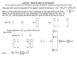
Lecture Density Matrix Formalism A tool used to describe the state of a spin ensemble, as well as its evolution in time. The expectation value X-component of the magnetic moment of nucleus A: Where is the wave function and is a linear combination of the eigenstates of the form:

Lecture Density Matrix Formalism
E N D
Presentation Transcript
Lecture Density Matrix Formalism A tool used to describe the state of a spin ensemble, as well as its evolution in time. The expectation value X-component of the magnetic moment of nucleus A: Where is the wave function and is a linear combination of the eigenstates of the form: Where |n> are the solution of the time-independent Schroedinger equation. The “bra, <n| and “ket, |n>” , and the angular momentum operator can be written in the matrix form as: IXA = Thus:
The N2 terms can be put in the matrix form as follow: Where = d*mn, i.e. D is a Hermitian matrix Thus, = NoA The angular momentum operators for spin ½ systems are: For spin 1: For a coupled A(½ )X(½) system
Using the expression: = -(4/p)MoA(d11/2 – d22/2 + d33/2 – d44/2) Where And Remember and Similarly: and In modern NMR spectrometers we normally do quadrature detection, i.e. For nucleus A we have: Similarly, for nucleus X: The density matrix at thermal equilibrium: Thus, if n ≠ m and Evolution of the density matrix can be obtained by solving the Schoedinger equation to give: Effect of radiofrequency pulse: Where R is the rotation matrix
For an isolated spin ½ system: For A(½)X(½) system:
Density matrix description of the 2D heteronuclear correlated spectroscopy (uncoupled) (coupled) For a coupled two spin ½ system, AX there are four energy states (Fig. I.1); (1) |++>; (2) |-+>; (3) |+->, and (4) |-->. The resonance frequencies for observable single quantum transitions (flip or flop) among these states are: 1QA: 12 (|++> |-+>)= A + J/2; 24 (|-+> |-->)= X - J/2; 1Qx: 13 (|++> |+->)= X + J/2; 34 (|+-> |-->)= A - J/2; Other unobservable transitions are: Double quantum transition 2QAX (Flip-flip): |++> |--> (flop-flop): |--> |++> Zero quantum transitions (flip-flop): ZQAX: |+-> |-+> or |-+> |+-> Density matrix of the coupled spin system is shown on Table I.1. The diagonal elements are the populations of the states. The off-diagonal elements represent the probabilities of the corresponding transitions. (1) (2) (3) (4)
1. Equilibrium populations: At 4.7 T: For a CH system, A = 13C and X = 1H and x 4C q 4p Thus, Hence: where 4 Unitary matrix Therefore,
2. The first pulse: where • The pulse created 1QX (proton) (non-vanishing d13 and d24) 3. Evolution from t(1) to t(2):
To calculate D(2) we need to calculate the evolution of only the non-vanishing elements, i.e. d13 and d24 in the rotating frame. are the rotating frame resonance frequencies of spin A and X, respectively, and TrH is the transmitter (or reference) frequency. Hence: where B* and C* are the complex conjugates of B and C, respectively. 4. The second pulse (rotation w.r.t. 13C): D(3) = R180XCD(2)R-1180XC = 5. Evolution from t(3) to t(4): ( is lab frame and is rotating frame resonance frequency) Substituting B and C into the equations we get: J is absent Decoupled due to spin echo sequence +
6. The role of 1 (Evolution with coupling): and Let = 1/2J and We have: Let Thus, 7. The third and fourth pulses: Combine the two rotations into one and
D(7) = R180XCD(2)R-1180XC = D(5) • Proton magnetization, d13 and d24 has been transferred to the carbon magnetization, d12 and d34 with and 8. The role of 2: Signal is proportional to d12+d34 we can’t detect signal at this time otherwise s will cancel out. The effect of 2 is as follow (Only non-vanishing elements, d12 and d13 need to be considered: • Hence: • For 2 = 0 the terms containing s cancel. • For 2 = 1/2J we have: 9. Detection: During this time proton is decoupled and only 13C evolve. Thus,
As described in Appendix B, in a quasrature detectin mode the total magnetization MTC is: • if we reintroduce the p/4 factor. • Thus, • This is the final signal to be detected. The 13C signal evolve during detection time, td at a freqquency Hand is amplitude modulated by proton evolution The. Fourier transform with respect to td and te results in a 2D HETCOR spectrum as shown on Fig. I.3a. The peak at -H is due to transformation of sine function due to The negative peak can be removed by careful placing the reference frequency and the spectral width or by phase cycling. • If there is no 180o pulse during te we will see spectrum I.3.b • If there is also no 1H decoupling is during detection we will get spectrum I.3.c.