Advanced Techniques in 3D Model Acquisition and Reconstruction
960 likes | 991 Vues
Explore cutting-edge methods in 3D model acquisition and reconstruction. Learn about range acquisition, alignment, and merging processes, including ICP variants and point selection strategies. Delve into matching techniques, such as closest point, normal shooting, and projection-based methods. Enhance your understanding of optimizing error metrics and minimizing transformations for precise model alignment.

Advanced Techniques in 3D Model Acquisition and Reconstruction
E N D
Presentation Transcript
3D photography (II) Digital Visual Effects, Spring 2005 Yung-Yu Chuang 2005/5/25 with slides by Szymon Rusinkiewicz, Richard Szeliski, Steve Seitz and Brian Curless
Announcements • Final project will be online tomorrow • Proposal presentation on next Wednesday • I will send out your current grades by next Wednesday • Scribe (SIGGRAPH 2005, CVPR 2005, readings) • Schedule for the next few weeks • 6/1 proposal • 6/8 making face/human • 6/15 random topics • 6/28 final project presentation
Outline • Range acquisition techniques • Full model reconstruction • ICP • Volumetric reconstruction • Systems, projects and applications • Final project
Range acquisition taxonomy mechanical (CMM, jointed arm) inertial (gyroscope, accelerometer) contact ultrasonic trackers magnetic trackers industrial CT rangeacquisition transmissive ultrasound MRI radar non-optical sonar reflective optical
Range acquisition taxonomy shape from X: stereo motion shading texture focus defocus passive opticalmethods active variants of passive methods Stereo w. projected texture Active depth from defocus Photometric stereo active time of flight triangulation
Passive approaches stereo space carving
Active approaches Cyberware whole body scanner shadow scanning
3D Model Acquisition Pipeline 3D Scanner
View Planning 3D Model Acquisition Pipeline 3D Scanner
View Planning Alignment 3D Model Acquisition Pipeline 3D Scanner
View Planning Alignment Merging 3D Model Acquisition Pipeline 3D Scanner
Problem • Align two partially-overlapping meshesgiven initial guessfor relative transform
Aligning 3D data • If correct correspondences are known,it is possible to find correct relative rotation/translation
Aligning 3D data • How to find corresponding points? • Previous systems based on user input,feature matching, surface signatures, etc.
Aligning 3D data • Alternative: assume closest points correspond to each other, compute the best transform…
Aligning 3D Data • … and iterate to find alignment • Iterated Closest Points (ICP) [Besl & McKay 92] • Converges if starting position “close enough“
ICP variants • Variants on the following stages of ICPhave been proposed: • Selecting source points (from one or both meshes) • Matching to points in the other mesh • Weighting the correspondences • Rejecting certain (outlier) point pairs • Assigning an error metric to the current transform • Minimizing the error metric
ICP variants • Selecting source points (from one or both meshes) • Matching to points in the other mesh • Weighting the correspondences • Rejecting certain (outlier) point pairs • Assigning an error metric to the current transform • Minimizing the error metric
Selecting source points • Use all points • Uniform subsampling • Random sampling • Normal-space sampling • Ensure that samples have normals distributedas uniformly as possible
Normal-space sampling Uniform Sampling Normal-Space Sampling
Random sampling Normal-space sampling Normal-space sampling • Conclusion: normal-space sampling better for mostly-smooth areas with sparse features
ICP variants • Selecting source points (from one or both meshes) • Matching to points in the other mesh • Weighting the correspondences • Rejecting certain (outlier) point pairs • Assigning an error metric to the current transform • Minimizing the error metric
Matching • Matching strategy has greatest effect on convergence and speed • Closest point • Normal shooting • Closest compatible point • Projection
Find closest point in other mesh Closest-point matching Closest-point matching generally stable, but slow and requires preprocessing
Project along normal, intersect other mesh Normal shooting Slightly better than closest point for smooth meshes, worse for noisy or complex meshes
Closest compatible point • Can improve effectiveness of both of the previous variants by only matching to compatible points • Compatibility based on normals, colors, etc. • At limit, degenerates to feature matching
Projection to find correspondences • Finding closest point is most expensive stage ofthe ICP algorithm • Idea: use a simpler algorithm to find correspondences • For range images, can simply project point [Blais 95]
Projection-based matching • Slightly worse performance per iteration • Each iteration is one to two orders of magnitude faster than closest-point
ICP variants • Selecting source points (from one or both meshes) • Matching to points in the other mesh • Weighting the correspondences • Rejecting certain (outlier) point pairs • Assigning an error metric to the current transform • Minimizing the error metric
ICP variants • Selecting source points (from one or both meshes) • Matching to points in the other mesh • Weighting the correspondences • Rejecting certain (outlier) point pairs • Assigning an error metric to the current transform • Minimizing the error metric
Point-to-plane error metric • Using point-to-plane distance instead of point-to-point lets flat regions slide along each other [Chen & Medioni 91]
High-speed ICP algorithm • ICP algorithm with projection-based correspondences, point-to-plane matchingcan align meshes in a few tens of ms.(cf. over 1 sec. with closest-point)
Range processing pipeline • Steps 1. manual initial alignment 2. ICP to one existing scan 3. automatic ICP of all overlapping pairs 4. global relaxation to spread out error 5. merging using volumetric method
Range processing pipeline • Steps 1. manual initial alignment 2. ICP to one existing scan 3. automatic ICP of all overlapping pairs 4. global relaxation to spread out error 5. merging using volumetric method
Volumetric integration (Curless and Levoy, Siggraph´96) range surfaces signed distance to surface volume weight (~accuracy) distance depth sensor surface1 • use voxel space • new surface as zero-crossing • (find using marching cubes) • least-squares estimate • (zero derivative=minimum) surface2 combined estimate
Isosurfacing: marching cubes First 2D, marching squares