Cartesian Computations: Architectural Trends and Technology Innovations
Explore the intersection of architectural trends and technology advancements in Cartesian computations, highlighting the balance between computation costs and data movement challenges. Dive into examples, implementations, and analyses that shape modern computational approaches.

Cartesian Computations: Architectural Trends and Technology Innovations
E N D
Presentation Transcript
Larry Carter with thanks to Bowen Alpern, Jeanne Ferrante, Kang Su Gatlin, Nick Mitchell, Michelle Strout Cartesian Computations Cartesian Computations
Outline • Architectural trends • Computation is (almost) free • Data movement and memory aren’t • Cartesian computations • Examples • Static, tidy and lazy implementations • Analysis of Cartesian computations • Computation density and temp data ratio • Some theorems • Application to examples Cartesian Computations
Technology trends Everything’s getting smaller Energy consumption limits computation speed Need to keep chip from melting Electricity costs are non-trivial! Energy is dominated by cost to move data In 32 nm technology (available today): 0.1 pJ (picoJoule) to add two 32-bit numbers 2 pJ to move a 32-bit number 1 mm on chip 320 pJ to move a 32-bit number onto or off a chip these numbers may be reduced by 10x with heroic methods, e.g. very low power&speed feature width chip light atom m mm µm nm Å Cartesian Computations
Computation is (almost) free On a 20 x 20 mm chip, you can fit: 1,000,000 32-bit adders, … or … 256 MB fast memory (SRAM) Memory is what takes up area For 100 Watts of power, you can Perform 1015 additions per second (one petaOp), … or … Read data from DRAM at 128 GB/sec Memory and moving data is what consumes power Cartesian Computations
Proc L1 L2 (Super)computer architecture Core = CPU + caches Chip = bunch of cores High bandwidth interconnect Node = bunch of chips + DRAM Tb/sec bandwidth between chips Less bandwidth to memory System = bunch of nodes Switch or grid connection OK bandwidth for block transfer P P L1 L1 L2 L2 P P L1 L1 L2 L2 DRAM Cartesian Computations
Models of computation RAM PRAM Proc Memory Memory Proc Proc Proc Proc Memory Cartesian Computations
The point being … (P)RAM analysis counts arithmetic operations, ignoring cost of memory accesses and data movement Real costs, both time and energy, are dominated by memory accesses and data movement These costs vary by over 100x depending on where data goes Algorithm analysis should focus on data movement! The rest of this talk will study data movement for a common class of scientific computation kernels not even considering disk Cartesian Computations
Outline • Architectural trends • Computation is (almost) free • Data movement and memory aren’t • Cartesian computations • Examples • Static, tidy and lazy implementations • Analysis of Cartesian computations • Computation density and temp data ratio • Some theorems • Application to examples Cartesian Computations
An incomplete taxonomy of kernels Compute intensive E.g. well-tuned matrix multiply, seismic migration, … Runtime is dominated by core speed Streaming applications E.g. simple encoding, scanning, one pass of quicksort, … Runtime dominated by sequential access to memory Dynamic data structures E.g. binary search trees, quadtrees, graph algorithms Runtime dominated by random access to memory and … Cartesian Computations
Cartesian computation Given large data structures A and B A generates temporary data T, which updates B For each chunk of A and B, there ’s a “tile” of computation There may be data dependences, but we’ll assume that reordering is possible. In a uniform Cartesian computation, for all tiles of a given size, the amount of computation is roughly the same. A B Cartesian Computations
A messy detail For very small tiles, the uniformity assumption fails How small is “very small” depends on the computation Most very small tiles will have no temp data or work If we only execute non-empty very small tiles, there is a savings in communication costs. But using very small tiles requires much more communication than using large tiles • In this talk, we assume that such a strategy is too expensive! • We also leave the open the problem of non-uniform distributions. Cartesian Computations
Sparse matrix-vector product y = Mx A = input vector (x), B = output vector (y) T might be pairs of the form {i, Mij xj} Matrix M could be: known implicitly (e.g. regular grid), or streamed in from local memory stored in order of use A tile is a rectangular subset of M The memory characteristics of y = Mx depend on the density & distribution of nonzeros depend on the implementation x y * * * * * M Cartesian Computations
A different (?) example 3 1 4 1 5 9 2 6 5 3 5 8 9 7 Histogram (from NAS Integer Sort Benchmark) For i=1 to numkeys Tally[Key[i]]++ Key is A;Tally is B; Temp data is indices into tile’s subset of tally Transpose, Bit Reversal (used in FFTs), and other Permutations are similar 5 Key 6 5 0 1 2 3 4 5 6 7 8 9 Tally Cartesian Computations
Generalization: Map-Reduce Input A is a set of (key,value) pairs Distributed by “key” in big computer “Map” takes each (k,v) to a list {(k1,v1), (k2,v2), … } Resulting data is sorted according to new keys Sj = {v | (kj, v) comes from Map} This is intermediate data of Cartesian computation “Reduce” is applied to each Sj, producing a new pair (kj, Reduce(Sj)) (or more generally, any number of new pairs) This is output set B Cartesian Computations
In general … In a uniform Cartesian computation, • chunks of A are used to generate temporary data may need extra “one-time” data too • chunks of B consume the temporary data N.B. the intermediate values of B are not called temp data • every chunk of A generates data for every chunk of B Program for executing Cartesian computations: for each “architectural unit” (cache, core, chip, node, …), choose • tile size and shape • whether to move temp data or to move chunks of A and/or B • how to use multiple processors and share memory Cartesian Computations
Implementing Cartesian computations Tidy Implementation • Temp data is consumed as soon as it is generated • relevant chunks of both A and B must be in local memory • A and B chunks are copied or moved so each is together at some time Temp data doesn’t move; but each bit of A and B may move many times • particularly if the tiles are small Lazy Implementation • Bring bits of A into a processor; generate temp data • Move temp either: • To another processor, or • To some level of cache memory • Consume temp data where or when appropriate chunk of B is available Temp data moves, but A and B may move less than for tidy program Cartesian Computations
Two types of lazy implementation • Static partitioning: • Partition B among memory of all “architectural units” B must fit in totality of these memories • Stream A in a few bits at a time, generate temp data and send it to unit owning appropriate chunk of B A and B only moved once Temp data may need to travel long distance Aside: we could swap the roles of A and B. • Bucket tiling: • Stream A in, generate & store temp data in local memory Store A in bucket depending on which chunk of B will consume it • Later, bring B in a chunk at a time, consume temp data • Repeat the above until done A and/or B may move in & out many times. Cartesian Computations
Bucket Tiling Example: histogram For i=1 to numkeys Tally[Key[i]]++ becomes … For ii=0 to numKeys by chunk_size // Break set of Keys into chunks Bend[*] = 0 For i=ii to ii + chunk_size // Put keys into buckets k = Key[i]>>16 // (indexed by high bits) Temp[k][Bend[k]++] = Key[i] && mask For k = 0 to numBuckets // Process each bucket For i = 0 to Bend[k] Tally[(k<<16)+Temp[k][i]]++ Choosechunk_size so that Temp fits in L2 cache; Choose “16” so random accesses to Tally are in L1 cache Code ran 3x faster (very old experiment) Cartesian Computations
Hybrid implementations Many variants are possible: Different strategies at different levels of granularity E.g. tidy implementation within node; lazy within chip If a chunk of A (or B) is needed in several places, it can either move from place or there can be duplicate copies If B has copies, they need to be combined at end. Different strategies for different regions E.g., if (non-uniform) problem has dense regions, use static partitioning but duplicate denser parts of A and/or B to reduce communication Cartesian Computations
Outline • Architectural trends • Computation is (almost) free • Data movement and memory aren’t • Cartesian computations • Examples • Static, tidy and lazy implementations • Analysis of Cartesian computations • Computation density and temp data ratio • Some theorems • Application to examples Cartesian Computations
Data movement in Cartesian computations Focus on moving of A, B, and temp data … ignore other data … into an architectural component cache, core, chip, node Same analysis for sequential or parallel execution. Useful metrics: Bits moved into component gives approximate energy or power requirement (power = energy/time) ignores difference between moving from DRAM vs. another chip ignores difference between near and distant network moves Computation/communication ratio = ops/sec ÷ bits/sec = speed ÷ bandwidth DRAM Cartesian Computations
Quantifying data movement Measure chunks of A and B in bits Tiles area is measured in “square bits” In a uniform problem, tile area is proportional to work Define compute density = work/bits2 (e.g. floatOps/bit2) Measure temp data in bits Suppose an a x b tile generates t bits temp data. Define (temp) data densityd = t/ab (d is “bits/bit2”) In a uniform problem, d is independent of tile choice Suppose all temp data is moved off-chip (or off-core or off-node): (almost happen in static partitioning – occasionally B is local) bits moved = abd compute speed / bandwidth ≤ /d Cartesian Computations
y = Mx example Suppose x and y are 64-bit floats. Suppose 1/400 of matrix entries are non-zero similar to NAS cg class B benchmark = 2 floatOps/(400 x 64 bits x 64 bits) ≈ 1.2 x 10⁻⁶ floatOp/bit2 Suppose temp data is {64 bit float, 32-bit index} d = 96 bits/(400 x 64 x 64 bit2) ≈ 58 x 10-6 bit-1 Note: /d = 1 floatOp/48 bits Typical supercomputer has only 4 bit DRAM bandwidth per floatOp x y * * * * * M ≈ compute/communication for static partitioning Cartesian Computations
Lower bound on tidy implementation Recall: the intermediate data is consumed immediately in the same component as it is produced. And, every square bit of Ax B co-resides in memory at some time Theorem: If a machine component with memory capacity c executes an ax b tile tidily, a>c and b>c, then ab/c bits must move into the component during the computation, even if the memory contained data at the start. Note: This is better than abd (static partitioning) if 1/c < d Corollary: computation speed ≤ xmemory capacity x bandwidth Cartesian Computations
Proof (if memory is initially empty): Assign a penny to each square bit (i,j) in tile total of ab pennies The first time i and j are in the same core, give penny to whichever load operation brought i or j in later no load can get more than c pennies Thus, there must be at least ab/c load operations. Proof (general case): Messy. Cartesian Computations
Upper bound on tidy implementations Tiling an a x b Cartesian problem: For all chunks Bi of B of size c(1-) Move Bi into local memory Stream through all nibbles of A of size Execute tile nibble x Bi B moves into component once b bits of B are moved At most b/c(1-) + 1 chunks of Bab/c(1-) + a bits of A moved Temp data is always local. Total: ab/c(1-) + a + b bits For large a and b and small , this is about ab/c matching the lower bound Cartesian Computations
Hierarchical tiling example B Partition A among DRAM of nodes Each cache-sized chunk of B makes a tour of all nodes When at a node, chunk resides in cache of one core local part of A streams into core relevant tile is executed Data movement of B between nodes is ab/ DRAM size corresponds to horizontal lines in picture Movement of A into cores is ab / cache size vertical lines in picture A DRAM size Cache size Cartesian Computations
Lower bound for bucket tiling Recall: Bucket tiling has only two operations: move bits of A into component, generate temp data move bits of B into component, consume temp data Theorem: A bucket tiled uniform Cartesian computation, where temp data is stored in a component with memory capacity c, moves at least ab(2d/c)½bits of A and B into the component. Proof: See Carter & Gatlin, FOCS ’98 But (d/c)½ is the geometric mean of d and 1/c, so this is worse than abd (static partitioning) or ab/c (tidy) or both. Possible advantage over static partitioning: If B doesn’t fit in sum of local memories, can’t static partition Bucket tiling communication is to nearest neighbor tiling static partitioning Cartesian Computations
Upper bound on bucket tiling Partition space into mxn tiles Entire axb problem needs ab/mn tiles Tile generates mnd bits of temp data; must be ≤ c For each tile: Movembits of A into node and create temp data from it Consume temp data by moving and updating nbits of B m+n bits of A and B moved per tile (temp data stays in cache) Data movement is minimized if m = n = (c/d)½ so total communication = ab/(c/d) x 2(c/d) ½ = 2ab (d/c)½ 6x6 tile needs 12 bits moved (3 bits/point) 4x9 tile needs 13 bits moved Cartesian Computations
(Theoretically) better implementation Form triangular tile with side m m(m-1)d/2 temp data; must be ≤ c; so m (2c/d)½ Slide tile along by deleting one column, placing one row communication = ab (2d/c)½ sqrt(2) times better (4 vs 3 points/bit moved in example) matches lower bound generate delete Cartesian Computations
Which implementation is best? N e t w o r k Each core has cache of size c1 Node has memory of size c2 >> c1 a = |A| > c2, b = |B| > c2 d = temp data ratio DRAM Cartesian Computations
Sparse Matrix-Vector example Each core has cache of size c1 Node has memory of size c2 >> c1 a = |A| > c2, b = |B| > c2 d = 58 x 10-6 (2KB)-1 Cartesian Computations
Histogram example Key 5 Suppose A is 64-bit integers and B is 16-bit counters There’s one increment operation per row An a x b tile (a and b are bits) represents a/64 rows In a uniform problem, tile contains b/|B| of indices so tile has (a/64)x(b/|B|) = ab/64|B| “hits” = work/bit2 = (ab/64|B|)/ab = 1 / 64|B| adds/bit2 Suppose we need 32-bit indices for temp data (fewer bits are needed since index is limited in tile) d = t/ab = (ab/64|B|) x 32/ab = 1 / (2|B|) Note: /d = 1 add/32 bits (not at all surprising) 6 5 Tally |B| is size of B in bits ≈ compute/communication for static partitioning Cartesian Computations
Histogram example Each core has cache of size c1 Node has memory of size c2 >> c1 a = |A| > c2, b = |B| > c2 d = 1/(2b) Cartesian Computations
Conclusions, etc Computation is free A theory for data movement (analogous to a theory of computation) is needed for today’s architectures For Cartesian computations, we can relate the three orthogonal aspects of computers: computation speed bandwidth memory and choose algorithms accordingly Results are needed for other classes of computations ! And architectural features (e.g. sequential access)! Cartesian Computations
Backup slides Cartesian Computations
Implementing Cartesian computations (put some words here) B P1 P2 P3 P4 P1 1->2 1->3 1->4 P1 P2 P2 2->1 2->3 etc. A P3 P3 P4 P4 Static partitioning Tidy (tiling) Cartesian Computations
Algorithmic vs. memory analysis • MergeSort or QuickSort • O(N lg N) operations • Sequential memory access • BucketSort or CountSort • O(N) operations • Random memory access Cartesian Computations
Algorithmic vs. memory analysis • Sandia study of Linear Algebra algorithms Millions of floating point ops needed for sample problem • 1950: 1,000,000,000,000 Mops (Cramer’s rule) • 1965: 10,000,000 Mops (Gaussian Elimination) • 1975: 300 Mops (Gauss-Seidel) • 1985: 8 Mop (Conjugate Gradient) • Each algorithmic improvement results in less locality in memory references. Cartesian Computations
Integer Sort Example • Loop from NAS IS benchmark For i=1 to numkeys Tally[Key[i]]++Random access to Tally (BAD) • Bucket-tiling* For i=1 to numkeys // Count keys per bucket Bcount[Key[i]>>12]++ Bcount in cache (GOOD); Key is sequential (OK) For k=1 to maxKey>>12 // Find bucket end points Bend[k] = Bend[k-1]+Bcount[k] Bend fits in cache (GOOD) For i=1 to numkeys // Put keys into buckets Temp[Bend[Key[i]>>12]++] = Key[i] Bend in cache; Key and Temp are sequential (OK) For i=1 to numkeys // Count keys Tally[Temp[i]]++ Active parts of Tally stay in cache (GOOD); Temp OK Bottom Line: Code is over 2 times faster (on IBM RS6000). *Alpern & Carter ‘94, “Towards a Model for Portable Parallel Performance” Cartesian Computations
Inspector – Executor paradigm • Introduced by Chaos Group at U. Md. (led by Joel Saltz) e.g. 1995 TPDS paper • “Inspector” is runtime code that: • Iterates through loops without executing, records information about data access order • Reorders data in arrays or chooses new execution order • Generates new index arrays • “Executor” is (modified) code • Does the actual computation • Uses reordered data and index arrays Cartesian Computations