Early work in intelligent systems
Explore the groundbreaking contributions of Alan Turing and Arthur Samuel in the early development of intelligent systems, including the Turing Machine and Genetic Programming, shaping the field of AI. Learn about their innovative approaches and the evolution of machine learning concepts.

Early work in intelligent systems
E N D
Presentation Transcript
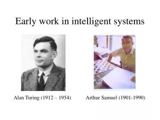
Early work in intelligent systems Alan Turing (1912 – 1954) Arthur Samuel (1901-1990)
Early work in intelligent systems • Alan Turing (1912 – 1954)Father of computer science, mathematician, philosopher, codebreaker (WW II), homosexual • The Turing Machine • The Turing Test (AI)
Early work in intelligent systems Alan Turing (1950):We cannot expect to find a good child-machine at the first attempt. One must experiment with teaching one such machine and see how well it learns. One can then try another and see if it is better or worse. There is an obvious connection between this process and evolution, by the identifications:Structure of the child machine = Hereditary materialChanges of the child machine = MutationsNatural selection = Judgment of the experimenter.
Early work in intelligent systems Arthur Samuel (1901-1990) • “How can computers learn to solve problems without being explicitly programmed? In other words, how can computers be made to do what is needed to be done, without being told exactly how to do it?" (1959) • “The aim is to get machines to exhibit behavior, which if done by humans, would be assumed to involve the use of intelligence.” (1983)
Genetic Programming • Breed a population of computer programs to solve a given problem • An extension of genetic algorithms • Selection, crossover, mutation
Preparatory Steps John Koza: the human user supplies: • The set of terminals (e.g., the independent variables of the problem, zero-argument functions, and random constants) (2) The set of primitive functions for each branch of the program to be evolved (3) The fitness measure (4) The parameters for controlling the run (5) The termination criteria
1. Terminal Set • External inputs to the program • Numerical constants (problem dependent?) • , e, 0, 1, … , random numbers, …
2. Function Set • Arithmetic functions • Conditional branches (if statements) • Problem specific functions (controllers, filters, integrators, differentiators, circuit elements, …)
3. Fitness Measure • The GP measures the fitness of each individual (computer program) • Fitness is usually averaged over a variety of different cases • Program inputs • Initial conditions • Different environments
4. Control Parameters • Population size (thousands or millions) • Selection method • Crossover probability • Mutation probability • Maximum program size • Elitism option
5. Termination Criterion • Maximum number of generations / real time • Convergence of highest / mean fitness • …
Initialization Max((* x x) (+ x (* 3 y))) Prefix notation (Lisp) Max(x*x, x+3*y) • Nodes (points, functions) • Links, terminals
Program Tree (+ 1 2 (IF (> TIME 10) 3 4)) If Time > 10 then x = 3 elsex = 4 Solution = 1 + 2 + x
Mutation • Select one individual probabilistically • Pick one point in the individual • Delete the subtree at the chosen point • Grow a new subtree at the mutation point in same way as for the initial random population • The result is a syntactically valid executable program
Crossover • Select two parents probabilistically based on fitness • Randomly pick a node in the first parent (often internal nodes 90% of the time) • Independently randomly pick a node in the second parent • Swap subtrees at the chosen nodes
Reproduction • Select an individual probabilistically based on fitness • Copy it (unchanged) into the next generation of the population (cloning)
Example Generate a computer program with one input x whose output equals the given data y ( y = x2+x+1 )
Fitness Evalution x+1 x2+1 2 x 0.67 1.00 1.70 2.67
Reproduction • Copy (a), the most fit individual • Mutate (c)
Interpreting a program tree { – [ + ( – 3 0 ) ( – x 1 ) ] [ / ( – 3 0 ) ( – x 2 ) ] } What does this evaluate as? What are the terminals, functions, and lists?
Interpreting a program tree { – [ + ( – 3 0 ) ( – x 1 ) ] [ / ( – 3 0 ) ( – x 2 ) ] } [ (3 – 0) + (x – 1) ] – [ (3 – 0) / (x – 2) ] • Terminals = { 3, 0, x, 1, 2} • Functions = { –, +, / } • Lists = ( – 3 0 ), [ + ( – 3 0 ) ( – x 1 ) ], …
Interpreting a program tree recursion \Re*cur"sion\ (-sh?n), n. [L. recursio.] See recursion. factorial ( n ) if n = = 0 then return 1 else return n * factorial (n – 1)
Interpreting a program tree Recursive function EVAL: if EXPR is a list then // i.e., delimited by parentheses PROC = EXPR(1) VAL = PROC [ EVAL(EXPR(2)), EVAL(EXPR(3)), …] else // i.e., EXPR is a terminal if EXPR is a variable or constant then VAL = EXPR else // i.e., EXPR is a function with no arguments VAL = EXPR ( ) end end
GP Inventions • Two patents filed by Keane, Koza, and Streeter on July 12, 2002 • Creation of Tuning Rules for PID Controllers that Outperform the Ziegler-Nichols and Åström-Hägglund Tuning Rules • Creation of 3 Non-PID Controllers that Outperform a PID Controller that uses the Ziegler-Nichols or Åström-Hägglund Tuning Rules
X band antenna – Jason Lohn, NASA Ames Wide beamwidth for a circularly polarized wave Wide bandwidth GP for Antenna Design
GP Computational Effort • Human brain 1012 neurons 1 msec 1015 operations per second 1 peta-op = 1 brain second (B-sec) • Keane, Koza, Streeter patents:
When should you use GP? • Problem involving many variables that are interrelated in highly nonlinear ways • Relationships among variables is not well understood • Discovery of the size and shape of the solution is a major part of the problem • “Black art” problems (controller tuning) • Areas where you have no idea how to program a solution, but you know what you want
When should you use GP? • Problems where a good approximate solution is satisfactory • Design • Control and estimation • Bioinformatics • Classification • Data mining • System identification • Forecasting
When should you use GP? • Areas where large computerized databases are accumulating and computerized techniques are needed to analyze the data • genome, protein, microarray data • satellite image data • astronomical data • petroleum databases • medical records • marketing databases • financial databases
Schema Theory for GP • The # symbol represents “don’t care” • Example: H = ( + ( –# y ) # ) instances are: ( + ( – x y ) x ) → ( x – y ) + x ( + ( – x y ) y ) → ( x – y ) + y ( + ( – y y ) x ) → ( y – y ) + x ( + ( – y y ) y ) → ( y – y ) + y
Schema Theory for GP Example: H = ( + ( –# y ) # ) • o(H) = number of defined symbolso(H) = ? • Length N(H) = number of symbolsN(H) = ? • Defining length L(H) = number of links joining defined symbolsL(H) = ?
All these schema sample the program ( + ( – 2 x ) y )What are the schema defining length L, order o, and length N? + + – – – # # # Schema Theory for GP # # # # # 2 # # # 2 x x
L = 3 L = 2 L = 1 L = 0 o = 4 o = 2 o = 2 o = 1 N = 5 N = 5 N = 5 N = 5 + + – – – # # # Schema Theory for GP # # # # # 2 # # # 2 x x
+ – – 2 x 3 y Schema Theory for GP How many schema match a tree of length N ? For example, consider the program ( + ( – 2 x ) ( – 3 y ) )
Schema Theory for GP Definitions: • m(H, t) = number of schema H at generation # t • G = structure of schema H For example, if H = ( + ( –# y ) # ) then G = ( # ( # # # ) # )
Schema Theory for GP • m(H, t) = number of schema H at gen. # t • m(H, t+1/2) = number of schema selected for crossover / mutation • m(H, t+1) = number of schema after crossover / mutation • Fitness proportionate selection:m(H, t+1/2) = m(H, t) f(H, t) / fave
Schema Theory for GP Crossover: two ways for destruction of schema H • Program h H crosses with program g that has a different structure than G Event D1 • Program h H crosses with program g that has the same structure as G, but g H Event D2 Pr(crossover destruction) = Pr(D) = Pr(D1) + Pr(D2 )
+ + + + – – – – 2 x 3 y Crossover Destruction – Type 1 ( + ( – 2 x ) ( – 3 y ) ) ( + x y ) Crossover results in ( + y ( – 3 y ) ) ( + x ( – 2 x ) ) Both schema are destroyed y 3 y x y x 2 x
Crossover Destruction – Type 2 If h = (+ x y) H = ( # x y) and g = (g1 y x) H then crossover between the + and x gives: ( + y x ) and (g1 x y ) H, schema preserved But if h = (+ x y) H = ( + x #) and g = ( g1 y x) H then crossover between the + and x gives: ( + y x ) and (g1 x y ) H, schema destroyed (unless g1 = “+”)
Crossover Destruction – Type 1 Program h H crosses with program g that has a different structure than G Event D1 M = population size Pr(D1) = Pr(D | g G) Pr(g G) Pr(g G) = [M – m(G, t+1/2)] / M Pr(D | g G) = Pdiff
Crossover Destruction – Type 2 Program h H crosses with program g that has the same structure as G but g H Event D2 Pr(D2) = Pr(D | g G) Pr(g G) Pr(g G) = m(G, t+1/2) / M Pr(D | g G) = Pr(D | g H) Pr(g H | g G) Pr(g H | g G) = [ m(G, t+1/2) – m(H, t+1/2) ] / m(G, t+1/2)