Biologically-Based Risk Estimation for Radiation-Induced Chronic Myeloid Leukemia
60 likes | 207 Vues
This study explores a Bayesian approach to estimate the risk of chronic myeloid leukemia (CML) induced by radiation exposure, utilizing principles of Bayesian inference with multivariate normal distributions. The authors discuss the relationship between prior, likelihood, and posterior distributions, emphasizing the equivalence in forming posteriors. A Gibbs sampling method is used for computation, allowing for efficient estimation of model parameters. The findings highlight the importance of combining prior knowledge with observed data to improve risk assessments in radiation-related health issues.

Biologically-Based Risk Estimation for Radiation-Induced Chronic Myeloid Leukemia
E N D
Presentation Transcript
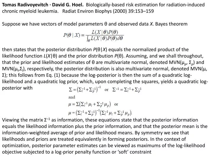
Tomas Radivoyevitch · David G. Hoel. Biologically-based risk estimation for radiation-induced chronic myeloid leukemia. RadiatEnviron Biophys (2000) 39:153–159 Suppose we have vectors of model parameters θ and observed data X. Bayes theorem then states that the posterior distribution P(θ|X) equals the normalized product of the likelihood function L(X|θ) and the prior distribution P(θ). Assuming, and we shall throughout, that the prior and likelihood estimates of θ are multivariate normal, denoted MVN(μp, Σp) and MVN(μl,Σl), respectively, the posterior distribution is also multivariate normal, denoted MVN(μ, Σ); this follows from Eq. (1) because the log-posterior is then the sum of a quadratic log-likelihood and a quadratic log prior, which, upon completing the squares, yields a quadratic log-posterior with Viewing the matrix Σ–1 as information, these equations state that the posterior information equals the likelihood information plus the prior information, and that the posterior mean is the information-weighted average of prior and likelihood means. By symmetry we see that likelihoods and priors are treated equivalently in forming posteriors. In the context of optimization, posterior parameter estimates can be viewed as maximums of the log-likelihood objective subjected to a log-prior penalty function or ‘soft’ constraint
Bayesian Inference using Gibbs Sampling (BUGS) version 0.5 Manual
Bayesian Inference using Gibbs Sampling (BUGS) version 0.5 Manual > LINE # name of this model in rjags JAGS model: model { for( i in 1 : N ) { Y[i] ~ dnorm(mu[i],tau) mu[i] <- alpha + beta * (x[i] - xbar) } tau ~ dgamma(0.001,0.001) sigma <- 1 / sqrt(tau) alpha ~ dnorm(0.0,1.0E-6) beta ~ dnorm(0.0,1.0E-6) } Fully observed variables: N Y x xbar
All in set V except v i.e. w In the liner model, the w are the yi and the product term is thus the likelihood term. The two v are mu and tau and the two parents of these, both of mu, are alpha and beta