Decision Modeling
Decision Modeling. Decision Analysis. Introduction. Decision analysis is the modeling of decision problems in which some or all of the model parameters are uncertain

Decision Modeling
E N D
Presentation Transcript
Decision Modeling Decision Analysis
Introduction • Decision analysis is the modeling of decision problems in which some or all of the model parameters are uncertain • Decision-making under risk represents those situations in which the decision maker is willing to assign probabilities to different outcomes • Decision-making under uncertainty represents those situations in which the decision maker is unwilling or unable to associate probabilities with different outcomes
Decision Tree Conventions • Decision trees are composed of nodes (circles, squares and triangles) and branches (lines). • The nodes represent points in time. • A decision node (a square) is a time when the decision maker makes a decision. • A probability node (a circle) is a time when the result of an uncertain event becomes known. • An end node (a triangle or no symbol at all) indicates that the problem is completed - all decisions have been made, all uncertainty have been resolved and all payoffs have been incurred.
Decision Tree Conventions • Time proceeds from left to right • Branches leading into a node (from the left) have already occurred • Branches leading out of a node (to the right) have not yet occurred • Branches leading out of a decision node represent the possible decisions; the decision maker can choose the preferred branch • Branches leading out of probability nodes represent the possible outcomes of uncertain events; the decision maker has no control over which of these will occur
Decision Tree Conventions • Probabilities are listed on probability branches • These probabilities are conditional on the events that have already been observed (those to the left) • The probabilities on branches leading out of any particular probability node must sum to 1 • Individual monetary values are shown on the branches where they occur, and cumulative monetary values are shown to the right of the end nodes • Two values are often found to the right of each node • The top one is the probability of getting to that end node • The bottom one is the associated monetary value
Newsvendor Model • A newsvendor can buy the Wall Street Journal newspaper for 40 cents a copy and sell them for 75 cents. • However, he must buy the papers before he knows how many he can actually sell. If he buys more papers than he can sell, he disposes of the excess at no cost. If he does not buy enough papers, he loses sales now and possibly in the future. • Suppose that the loss of future sales is captured by an opportunity cost of 50 cents per unsatisfied customer.
Newsvendor Model • The demand distribution is as follows: P0 = Prob{demand = 0} = 0.1 P1 = Prob{demand = 1} = 0.3 P2 = Prob{demand = 2} = 0.4 P3 = Prob{demand = 3} = 0.2 • Each of these four realized values of demand represent the states of nature with associated probabilities (please note that the probabilities add to one). The number of papers ordered is the decision. The returns or payoffs are as follows:
State of Nature (Demand) Decision 0 1 2 3 0 0 -50 -100 -150 1 -40 35 -15 -65 2 -80 -5 70 20 3 -120 -45 30 105 Payoff = 75(# papers sold) – 40(# papers ordered) – 50(unmet demand) Where 75¢ = selling price 40¢ = cost of buying a paper 50¢ = cost of loss of goodwill
Newsvendor Tree • Draw a decision tree for the newsvendor problem • See board for solution
Decision Tree Conventions • This decision tree illustrates the conventions for a single-stage decision problem, the simplest type of decision problem • In a single-stage decision problem all decisions are made first, and then all uncertainty is resolved • Later we will see multistage decision problems, where decisions and outcomes alternate • Once a decision tree has been drawn and labeled with the probabilities and monetary values, it can be solved easily
The Folding Back Procedure • The solution procedure used to develop this result is called folding back on the tree. Starting at the right on the tree and working back to the left, the procedure consists of two types of calculations. • At each probability node we calculate expected monetary value (EMV) and write it below the name of the node • At each decision node we find the maximum of the EMVs and write it below the node name • After folding back is completed we have calculated EMVs for all nodes
Exercise Rick O’Shea is an independent trucker operating out of Tucson. He has the option of either hauling a shipment to Denver or hauling a different shipment to Salt Lake City. If he chooses the shipment to Denver, he has a 90% chance of finding there a return shipment to Tucson. If he does not find a return shipment, he will return to Tucson empty. If he chooses the shipment to Salt Lake City, he has a 50% chance of finding a return shipment to Tucson. His payoffs are shown in the table below. Draw the decision tree for this model.
Sensitivity Analysis • Sensitivity analysis is always important in real decision analysis • If we had to construct a decision tree by hand, a sensitivity analysis would be virtually out of the question • We would have to re-compute everything each time we want to experiment with a set of values • In Excel, we can enter any values we wish in the input cells and watch how the tree changes • We can get more systematic information by developing and using one-way and two-way data tables
Sensitivity Analysis • The cell to analyze is usually the EMV cell at the far left of the decision tree but it can be any EMV cell • The entries of interest should be put in at the top of the spreadsheet and be referenced by absolute addresses • Use the table function to fill up the table for the missing entries • Once the table is created, it is possible to perform calculations and to create graphs of values of interest
Newsvendor Revisited • Draw a decision tree for the newsvendor problem in Excel • Create a one-way data table in which the opportunity cost of stock-outs vary from $0.00 to $1.50 in $0.10 increments • Compared to the base case of $0.50 stock-out cost, what is the change in policy if the stock-out cost is $0.00? What if the stock-out cost is $1.50?
Multistage Decisions • Sometimes, the decision process consists of making sequential decisions, some of which take place after nature has revealed its state • The decision tree retains the same basic structure, but probability nodes and decision nodes alternate from the root of the tree to the leaves • Often, an intermediate probability node represents the acquisition of additional information
Litigation Example Your company has been sued for patent infringement in two separate, but related, law suits. Your job is to devise a strategy for minimizing the expected cost of these suits. The first trial is scheduled for July 15 and the second trial for December 1. The preparation cost for each trial is $10,000, but is reduced to $6,000 for the second trial if the first case goes to trial. If you win the first trial, there is no penalty. If you lose, the penalty will be $200,000. Your estimate of the probability of winning is 0.5. However, if you choose to settle the case before it goes to trial, the penalty will be $100,000. You can settle the second case for $60,000 For the second trial, there are three possible outcomes: The judge finds the suit invalid; the suit is valid, but there was no infringement of the patent; and the suit is valid and there was an infringement. The payoffs and probabilities of these outcomes are listed in the following table: