Mobility and Chemical Potential
270 likes | 533 Vues
Mobility and Chemical Potential. Molecular motion and transport disucssed in TSWP Ch. 6. We can address this using chemical potentials. Consider electrophoresis: We apply an electric field to a charged molecule in water. The molecule experiences a force ( F = qE )

Mobility and Chemical Potential
E N D
Presentation Transcript
Mobility and Chemical Potential • Molecular motion and transport disucssed in TSWP Ch. 6. We can address this using chemical potentials. • Consider electrophoresis: • We apply an electric field to a charged molecule in water. • The molecule experiences a force (F = qE) • It moves with a constant velocity (drift velocity = u) • It obtains a speed such that the drag exactly opposes the electrophoretic force. No acceleration = steady motion. • u =qE·1/f where f is a frictional coefficient with units of kg s-1. • qE is a force with units of kg m s-2 giving u with the expected ms-1 velocity units. • Think of (1/f) as a mobility coefficient, sometimes written as µ. • u = mobility · force • We can determine the mobility by applying known force (qE) and measuring the drift velocity, u.
Mobility and Chemical Potential • Gradient of the chemical potential is a force. • Think about gradient of electrical potential energy: • Extending this to the total chemical potential: • where f is a frictional coefficient • (1/f) as a mobility coefficient
E + Mobility and Chemical Potential: Example - + Write down chemical potential as a function of position in this electrophoresis: If concentration (c) is constant througout: And the drift velocity is Potential (f) Position (x) What if c is not constant? Can the entropy term give rise to an effective force that drives motion? This is diffusion, and we can derive Fick’s Law (TSWP p. 269) from chemical potentials in this way.
Brownian Motion Brownian trajectory • Each vertex represents measurement of position • Time intervals between measurements constant • After time (t) molecule moves distance (d) • 2-dimensional diffusion: • <d2> = <x2> + <y2> = 4Dt • 3-dimensional diffusion: • <d2> = <x2> + <y2> + <z2> = 6Dt • In cell membrane, free lipid diffusion: • D ~ 1 µm2/s 1 “Random walk” µm t = 0 d 0 t = 0.5 s 0 1 µm A lipid will diffuse around a 10 µm diameter cell:
Diffusion: Fick’s First Law 1 • Jx = Flux in the x direction • Flux has units of #molecules / area • (e.g. mol/cm2) • Brownian motion can lead to a net flux of molecules in a given direction of the concentration is not constant. • Ficks First Law: µm 0 0 1 µm
Derivation of Fick’s First Law from Entropy of Mixing • Chemical potential of component 1 in mixture. • Net drift velocity (u) related to gradient of chemical potential by mobility (1/f) where f is frictional coefficient. • Flux (J1x) is simply concentration times net drift. • Einstein relation for the diffusion coefficient. • Entropy is the driving force behind diffusion.
Fick’s Second Law: The Diffusion Equation • Consider a small region of space (volume for 3D, area for 2D) • Jx(x) molecules flow in and Jx(x+dx) molecules flow out (per unit area or distance per unit time). N
Diffusion Example X X Jx Jx=0 [C] [C] A pore (100 nm2) opens in a cell membrane that separates the cell interior (containing micromolar protein concentrations) from the protein free exterior. How fast do the proteins leak out? (Assume D ~ 10-6 cm2/s)
Diffusion Question Thought problem: Axons of a nerve cell are long processes that can extend more than 1 meter for nerve cells that connect to muscles or glands. If an action potential starting in the cell body of the neuron proceeds by diffusion of Na+ and K+ to the synapse, how long does it take the signal to travel 1m? D25°C(Na+) = 1.5*10-5 cm2/sec D25°C(K+) = 1.9*10-5 cm2/sec Treat this as a 1D diffusion problem. <x2> = 2Dt
Transport Anisotropy Forces Law MW Dependence Property (Gradient) (Spherical Particles) Diffusion Concentration Diffusional D M-1/3 T, Pi Frictional Sedimentation Centrifugal Centrifugal s M-2/3 Velocity Acceleration Buoyant Frictional Sedimentation Centrifugal Centrifugal Equilibrium Acceleration, Buoyant Concentration Diffusional Viscosity Velocity Shear [] M Frictional Electrophoresis Electric Field Electrostatic Frictional Rotary Diffusion Shape Rotational Frictional
Thermal Motion: Maxwell-Boltzmann Distribution of Velocities Quantitative description of molecular motion Average translational molecular kinetic energy: k = Boltzmann constant = R/N0 = 1.38 x 10⁻²³ JK-1 molecule-1 Probibility of a molecule in a dilute gas having speed between u and u + du: Both T and m (mass) are in this equation.
Molecular Collisions • Speeds of molecules in gas phase can be very large. • ~ 500 m/s for O2 at 20 °C • Molecules do not travel far before colliding (at atm pressures) • z = number of collisions per second that one molecule experinces in a gas • N = molecules; V = total volume • s = diameter of spherical molecule (approx. size) • <u> = mean molecular speed
Molecular Collisions Number of collisions per second that one molecule experinces in a gas: Z = total number of collisions per unit volume per unit time: Number of molecules Prob. Of collision per molecule 2 molecules in each collision Volume
Mean Free Path The mean free path (l) is defined as the average distance a molecule travels between two successive collisions with other molecules. Brownian trajectory Compare to Brownian motion: Note that l ≠ d, in general. The vertices observed in Brownian trajectories may involve many collisions. The apparent “steps” result from the way we collect data. Mean free paths will generally be much shorter in condensed systems. 1 “Random walk” µm t = 0 d 0 t = 0.5 s 0 1 µm
Molecular Collisions and Reaction Kinetics • Chemical reactions that create a bond generally require molecular collisions. • Kinetic rate of these reactions should depend on the rate and energy of molecular collisions. • Collisions bring the reactants together • Kinetic energy from molecular motion enables reaction to cross over activation barrier. • This is not just translational motion, but also includes molecular vibrations, which are more important in large molecules like proteins.
Kinetics vs Equilibrium • Equilibrium configuration depends only on DG. • Free energy is a state function, path independent • In general, no rate information • Except for mixing, not reacting systems, where we found: • v is the drift velocity and f is the drag coefficient • We can solve this problem because we know the exact path • And we know the energy at each point along this path
Kinetics vs Equilibrium • For general chemical reactions we don’t know the exact path or mechanism. • Nor do we know the precise energy function. If we know all the details, physics will tell us the rate. Details generally not known for chemical reactions. Kinetics is a quantitative, but largely empirical, study of rates of reactions. It is useful because kinetic behavior reveals information about reaction mechanism. (e.g. signatures of life beyond Earth) Transition states reaction mechanisms Energy Reaction Coordinate
Rate Law & Definitions • Reaction velocity: v = dc/dt • Rate Law: Substances that influence the rate of a reaction grouped into two catagories • Concentration changes with time • Reactants (decrease) • Products (increase) • Intermediates (increase then decrease) • Concentration does not change • Catalysts (inhibitor or promoter) • Intermediates in a steady-state process • Components buffered by equilibrium with large reservoir • Solvent A --> C --> B Concentration Time
Order of a Reaction • Kinetic order of a reaction describes the way rate depends on concentration: A + B --> C • {m,n,q} are usually integers but not always • Order with respect to A is m etc. • Overall order of reaction is sum: m + n + q • Kinetic order depends on reaction mechanism, it is not determined by stoichiometry. • H2 + I2 -> 2HI Second order overall • H2 + Br2 -> 2HBr Complex
Zero-Order Reactions • Rate law: • Seen in some enzymatic reactions such as that of liver alcoholdehydrogenase: CH3CH2OH + NAD+ CH3CHO + NADH + H+ ethanol acetaldehyde LADH ethanol acetaldehyde Concentration NAD+ is buffered Enzyme is saturated Note: Reaction cannot be strictly zero order at all times. Time
First Order Reactions • Rate law: • Typical of unimolecular reaction mechanism A -> B • Rearrange and integrate Ln[A] Time [A]0 [A] Time
First Order Reactions: half-life and relaxation time • Half-life: Time required for half of the initial concentration to react • 1/2-life of 14C decay is 5770 years • Relaxation time [A]0 [A]0/2 Half-life Time [A]0 [A]0/e Time t
Second Order Reactions • Class I rate law: • Possible bimolecular mechanism A + A --> P • Example: RNA hybridization • General form • Separate variables and integrate A-A-G-C-U-U k2 2 A-A-G-C-U-U U-U-C-G-A-A Letting x be the amount of A that has reacted:
Second Order Reactions: Class I [A]0 [A]0/2 Half-life Time
Second Order Reactions: Class II • Class II reaction rate law for A + B --> P • First order with respect to either A or B • Second order overall • Some examples: NO(g) + O3(g) --> NO2(g) + O2(g) v = k2[NO][O3] H2O2 + 2Fe2+ + 2H+(excess) --> 2H2O + 2Fe3+ v = k2[H2O2][Fe2+ ] • Reactions of different stoichiometric ratios can exhibit class II kinetics.
Second Order Reactions: Class II General rate law: Letting x be the concentration of each species that has reacted: Integrating: Slope = ([A]0 - [B]0)·k2 Ln([A]/[B]) Time
Last Homework From TSWP: Ch6: 1, 3,13 + 12 & 24 (which cover sedimentation) Ch7: 1, 4, 10 (more problems may be added next week) From Class: A pore (100 nm2) opens in a cell membrane that separates the cell interior (containing micromolar protein concentrations) from the protein free exterior. How fast do the proteins leak out? (Assume D ~ 10-6 cm2/s) If an action potential starting in the cell body of the neuron proceeds by diffusion of Na+ and K+ to the synapse, how long does it take the signal to travel 1m? D25°C(Na+) = 1.5*10-5 cm2/sec D25°C(K+) = 1.9*10-5 cm2/sec Treat this as a 1D diffusion problem. <x2> = 2Dt