Multiple Regression
Multiple Regression. Here we consider more than one explanatory variable in the regression . Math form. The multiple regression form of the model is (the book has Greek letters): Yi = B 0 + B 1 x 1 + B 2 x 2 + … + e, where

Multiple Regression
E N D
Presentation Transcript
Multiple Regression Here we consider more than one explanatory variable in the regression.
Math form The multiple regression form of the model is (the book has Greek letters): Yi = B0 + B1 x1 + B2x2 + … + e, where B0 is the Y intercept of the line, Bi is the slope of the line in terms of xi, and e is an error term that captures all those influences on Y not picked up by the x’s. The error term reflects the fact that all the points are not directly on the line. So, we think there is a regression line out there that expresses the relationship between x’s and Y. We have to go find it. In fact we take a sample and get an estimate of the regression line. Note that in general we talk about p explanatory variables.
When we have a sample of data from a population we will say in general the regression line is estimated to be Ŷi = b0 + b1 x1 + b2x2 + …, where the ‘hat’ refers to the estimated, or predicted, value of Y. Once we have this estimated line we are right back to algebra. Ŷ values are exactly on the line. Now, for an each value of x we have data values, called Y’s, and we have the one value of the line, called Ŷ. This part of multiple regression is very similar to simple regression. But our interpretation will change a little.
Here we will consider an example where we believe the response variable of total US revenue for a movie is explained by the variables the budget used to make the movie, the opening weekend revenue, and the number of theaters the movie was viewed. The dollar values are measure in millions of dollars. A sample of 40 movies is used to infer about the population relationship between movies total revenue and the p = 3 explanatory variables. The multiple regression results are shown on the next screen.
F Test In a multiple regression, a case of more than one x variable, we conduct a statistical test about the overall model. The basic idea is do all the x variables as a package have a relationship with the Y variable? The null hypothesis is that there is no relationship and we write this in a shorthand notation as Ho: B1 = B2 = … =0. If this null hypothesis is true the equation for the line would mean the x’s do not have an influence on, or help explain, Y. The alternative hypothesis is that at least one of the beta’s is not zero, written H1: not all Bi’s = 0. Rejecting the null means that the x’s as a group are related to Y. The test is performed with what is called the F test. From the sample of data we can calculate a number called the F statistic and use this value to perform the test. In our class we will have F calculated for us because it is a tedious calculation.
F Under the null hypothesis the F statistic we calculate from a sample has a distribution similar to the one shown. The F test here is a one tailed test. The farther to the right the statistic we get in the sample is, the more we are inclined to reject the null because extreme values are not very likely to occur under the null hypothesis. In practice we pick a level of significance and use a critical F to define the difference between accepting the null and rejecting the null.
Area we make = alpha F Critical F To pick the critical F we have two types of degrees of freedom to worry about. We have the numerator and the denominator degrees of freedom to calculate. They are called this because the F stat is a fraction. Numerator degrees of freedom = number of x’s, in general called p. Denominator degrees of freedom = n – p – 1, where n is the sample size. As an example, if n = 40 and p = 3 we would say the degrees of freedom are 3 and 36 where we start with the numerator value. You would see from a book the critical F is 8.59 when alpha is .05. Many times the book also has information for alpha = .025 and .01.
Area we make = alpha =.05 here F 8.59 here In our example here the critical F is 8.59. If from the sample we get an F statistic that is greater than 8.59 we would reject the null and conclude the x’s as a package have a relationship with the variable Y. From the example in Excel we see the F stat is 81.61 and so the null hypothesis would be rejected in that case.
Area we make = alpha =.05 here F 8.59 here 81.61 P-value The computer printout has a number on it that means we do not even have to look at the F table if we do not want to. But, the idea is based on the table. Here you see 81.61 is in the rejection region. I have colored in the tail area for this number. Since 8.59 has a tail area = alpha = .05 here, we know the tail area for 81.61 must be less than .05. This tail area is the p-value for the test stat calculated from the sample and on the computer printout is labeled Significance F. In the example the value is 4.00135E-16. This is really small.
SOOOOOOO, Using the F table, Reject the null if the F stat > critical F in the table, or If the Significance F < alpha. If you can NOT reject the null then at this stage of the game there is no relation between the x’s and the Y and our work here would be done. So from here out I assume we have rejected the null. Next let’s move to the estimated regression line.
From the multiple regression output we see the coefficients section means the estimated regression line is estimated to be Ŷ = 53.7020 - 0.4988x1 + 3.2417x2 – 0.0012x3, where x1 = movie budget, x2 = first weekend revenue x3 = number of theaters. Each slope coefficient measures the mean change in Y per unit change in the particular x, holding constant the effect of the other x variables. What would you predict y to be (the yhat value) if x1 = 35, x2 = 78 and 3x = 2100? Did you get 286.49?
t tests – After the F test we would do a t test on each of the slopes similar to what we did in a simple linear regression case to make sure that each variable on its own has a relationship with y. We still reject the null of a zero slope when the p-value on the slope is less than alpha. If we can not reject the slope as being different from 0 we say that variable x3, for example, does not help predict or explain the response y, given that x1 and x2 are available for use in prediction (or x1 and x2 are also included in the model). In the example note that the number of theaters does not add to predicting given that the budget and opening weekend revenue are included. Let’s pause and look at a simple regression on total revenue and the number of theaters.
Note that here the number of theaters as a single variable does help to explain US sales.
r square R2 r square on the regression printout is a measure designed to indicate the strength of the impact of the x’s on y. The number can be between 0 and 1, with values closer to 1 meaning the stronger the relationship. r square is actually the percentage of the variation in y that is accounted for by the x variables. This is also an important idea because although we may have a significant relationship we may not be explaining much. But in our example of 3 explanatory variables we have an R2 = 0.871810415 So, a little more than 87% of the variation in sales is accounted for by the 3 variables as a group.

