An Introduction to Data Structures and Abstract Data Types
An Introduction to Data Structures and Abstract Data Types. The Need for Data Structures. Data structures organize data more efficient programs. More powerful computers more complex applications. More complex applications demand more calculations.

An Introduction to Data Structures and Abstract Data Types
E N D
Presentation Transcript
The Need for Data Structures Data structures organize data more efficient programs. More powerful computers more complex applications. More complex applications demand more calculations. Complex computing tasks are unlike our everyday experience.
Organizing Data Any organization for a collection of records can be searched, processed in any order, or modified. The choice of data structure and algorithm can make the difference between a program running in a few seconds or many days.
Efficiency A solution is said to be efficient if it solves the problem within its resource constraints. • Space • Time • The cost of a solution is the amount of resources that the solution consumes.
Selecting a Data Structure Select a data structure as follows: • Analyze the problem to determine the resource constraints a solution must meet. • Determine the basic operations that must be supported. Quantify the resource constraints for each operation. • Select the data structure that best meets these requirements.
Some Questions to Ask • Are all data inserted into the data structure at the beginning, or are insertions interspersed with other operations? • Can data be deleted? • Are all data processed in some well-defined order, or is random access allowed?
Data Structure Philosophy Each data structure has costs and benefits. Rarely is one data structure better than another in all situations. A data structure requires: • space for each data item it stores, • time to perform each basic operation, • programming effort.
Data Structure Philosophy (cont) Each problem has constraints on available space and time. Only after a careful analysis of problem characteristics can we know the best data structure for the task. Bank example: • Start account: a few minutes • Transactions: a few seconds • Close account: overnight
Abstract Data Types Abstract Data Type (ADT): a definition for a data type solely in terms of a set of values and a set of operations on that data type. Each ADT operation is defined by its inputs and outputs. Encapsulation: Hide implementation details.
Data Structure • A data structure is the physical implementation of an ADT. • Each operation associated with the ADT is implemented by one or more subroutines in the implementation. • Data structure usually refers to an organization for data in main memory. • File structure is an organization for data on peripheral storage, such as a disk drive.
Metaphors An ADT manages complexity through abstraction: metaphor. • Hierarchies of labels Ex: transistors gates CPU. In a program, implement an ADT, then think only about the ADT, not its implementation.
Logical vs. Physical Form Data items have both a logical and a physical form. Logical form: definition of the data item within an ADT. • Ex: Integers in mathematical sense: +, - Physical form: implementation of the data item within a data structure. • Ex: 16/32 bit integers, overflow.
Problems • Problem: a task to be performed. • Best thought of as inputs and matching outputs. • Problem definition should include constraints on the resources that may be consumed by any acceptable solution.
Problems (cont) • Problems mathematical functions • A function is a matching between inputs (the domain) and outputs (the range). • An input to a function may be single number, or a collection of information. • The values making up an input are called the parameters of the function. • A particular input must always result in the same output every time the function is computed.
Algorithms and Programs Algorithm: a method or a process followed to solve a problem. • A recipe. An algorithm takes the input to a problem (function) and transforms it to the output. • A mapping of input to output. A problem can have many algorithms.
Algorithm Properties An algorithm possesses the following properties: • It must be correct. • It must be composed of a series of concrete steps. • There can be no ambiguity as to which step will be performed next. • It must be composed of a finite number of steps. • It must terminate. A computer program is an instance, or concrete representation, for an algorithm in some programming language.
Mathematical Background Set concepts and notation. Recursion Induction Proofs Logarithms Summations Recurrence Relations
Estimation Techniques • Determine the major parameters that effect the problem. • Derive an equation that relates the parameters to the problem. • Select values for the parameters, and apply the equation to yield and estimated solution.
Estimation Example How many library bookcases does it take to store books totaling one million pages? Estimate: • Pages/inch • Feet/shelf • Shelves/bookcase
Algorithm Efficiency There are often many approaches (algorithms) to solve a problem. How do we choose between them? At the heart of computer program design are two (sometimes conflicting) goals. • To design an algorithm that is easy to understand, code, debug. • To design an algorithm that makes efficient use of the computer’s resources.
Algorithm Efficiency (cont) Goal (1) is the concern of Software Engineering. Goal (2) is the concern of data structures and algorithm analysis. When goal (2) is important, how do we measure an algorithm’s cost?
How to Measure Efficiency? Critical resources: Factors affecting running time: For most algorithms, running time depends on “size” of the input. Running time is expressed as T(n) for some function T on input size n.
Examples of Growth Rate Example 1: // Find largest value int largest(int array[], int n) { int currlarge = 0; // Largest value seen for (int i=1; i<n; i++) // For each val if (array[currlarge] < array[i]) currlarge = i; // Remember pos return currlarge; // Return largest }
Examples (cont) Example 2: Assignment statement. sum = 0; for (i=1; i<=n; i++) for (j=1; j<n; j++) sum++; }
Best, Worst, Average Cases Not all inputs of a given size take the same time to run. Sequential search for K in an array of n integers: • Begin at first element in array and look at each element in turn until K is found Best case: Worst case: Average case:
Which Analysis to Use? While average time appears to be the fairest measure, it may be difficult to determine. When is the worst case time important?
Faster Computer or Algorithm? What happens when we buy a computer 10 times faster?
Binary Search How many elements are examined in worst case?
Binary Search // Return position of element in sorted // array of size n with value K. int binary(int array[], int n, int K) { int l = -1; int r = n; // l, r are beyond array bounds while (l+1 != r) { // Stop when l, r meet int i = (l+r)/2; // Check middle if (K < array[i]) r = i; // Left half if (K == array[i]) return i; // Found it if (K > array[i]) l = i; // Right half } return n; // Search value not in array }
Other Control Statements while loop: Analyze like a for loop. if statement: Take greater complexity of then/else clauses. switch statement: Take complexity of most expensive case. Subroutine call: Complexity of the subroutine.
Analyzing Problems Upper bound: Upper bound of best known algorithm. Lower bound: Lower bound for every possible algorithm.
Space Bounds Space bounds can also be analyzed with complexity analysis. Time: Algorithm Space Data Structure
Space/Time Tradeoff Principle One can often reduce time if one is willing to sacrifice space, or vice versa. • Encoding or packing information Boolean flags • Table lookup Factorials Disk-based Space/Time Tradeoff Principle: The smaller you make the disk storage requirements, the faster your program will run.
Lists A list is a finite, ordered sequence of data items. Important concept: List elements have a position. Notation: <a0, a1, …, an-1> What operations should we implement?
List Implementation Concepts Our list implementation will support the concept of a current position. We will do this by defining the list in terms of left and right partitions. • Either or both partitions may be empty. Partitions are separated by the fence. <20, 23 | 12, 15>
List ADT template <class Elem> class List { public: virtual void clear() = 0; virtual bool insert(const Elem&) = 0; virtual bool append(const Elem&) = 0; virtual bool remove(Elem&) = 0; virtual void setStart() = 0; virtual void setEnd() = 0; virtual void prev() = 0; virtual void next() = 0;
List ADT (cont) virtual int leftLength() const = 0; virtual int rightLength() const = 0; virtual bool setPos(int pos) = 0; virtual bool getValue(Elem&) const = 0; virtual void print() const = 0; };
List ADT Examples List: <12 | 32, 15> MyList.insert(99); Result: <12 | 99, 32, 15> Iterate through the whole list: for (MyList.setStart(); MyList.getValue(it); MyList.next()) DoSomething(it);
List Find Function // Return true if K is in list bool find(List<int>& L, int K) { int it; for (L.setStart(); L.getValue(it); L.next()) if (K == it) return true; // Found it return false; // Not found }
Array-Based List Class (1) class AList : public List<Elem> { private: int maxSize; // Maximum size of list int listSize; // Actual elem count int fence; // Position of fence Elem* listArray; // Array holding list public: AList(int size=DefaultListSize) { maxSize = size; listSize = fence = 0; listArray = new Elem[maxSize]; }
Array-Based List Class (2) ~AList() { delete [] listArray; } void clear() { delete [] listArray; listSize = fence = 0; listArray = new Elem[maxSize]; } void setStart() { fence = 0; } void setEnd() { fence = listSize; } void prev() { if (fence != 0) fence--; } void next() { if (fence <= listSize) fence++; } int leftLength() const { return fence; } int rightLength() const { return listSize - fence; }
Array-Based List Class (3) bool setPos(int pos) { if ((pos >= 0) && (pos <= listSize)) fence = pos; return (pos >= 0) && (pos <= listSize); } bool getValue(Elem& it) const { if (rightLength() == 0) return false; else { it = listArray[fence]; return true; } }
Insert // Insert at front of right partition bool AList<Elem>::insert(const Elem& item) { if (listSize == maxSize) return false; for(int i=listSize; i>fence; i--) // Shift Elems up to make room listArray[i] = listArray[i-1]; listArray[fence] = item; listSize++; // Increment list size return true; }
Append // Append Elem to end of the list bool AList<Elem>::append(const Elem& item) { if (listSize == maxSize) return false; listArray[listSize++] = item; return true; }
Remove // Remove and return first Elem in right // partition AList<Elem>::remove(Elem& it) { if (rightLength() == 0) return false; it = listArray[fence]; // Copy Elem for(int i=fence; i<listSize-1; i++) // Shift them down listArray[i] = listArray[i+1]; listSize--; // Decrement size return true; }
Link Class Dynamic allocation of new list elements. // Singly-linked list node class Link { public: Elem element; // Value for this node Link *next; // Pointer to next node Link(const Elem& elemval, Link* nextval =NULL) { element = elemval; next = nextval; } Link(Link* nextval =NULL) { next = nextval; } };