Download

1 / 68
730 likes | 899 Vues
Positron Emission Tomography - training - IBRO CEERC Summer School 2005 Miklós Emri , Iván Valastyán, Gábor Opposits. PET Center University of Debrecen 2005. PET- method. Isotope preparation F 18 , O 15 , C 11 , N 13 Radiop h ar m a c on evaluation FDG, Metionine, F-dopa, Butanol. H 2 O

E N D
Positron Emission Tomography- training -IBRO CEERC Summer School 2005MiklósEmri , IvánValastyán, Gábor Opposits PET Center University of Debrecen 2005
PET-method • Isotope preparation • F18, O15, C11, N13 • Radiopharmacon evaluation • FDG, Metionine, F-dopa, Butanol. H2O • Imaging • Static-, dynamic, ECG gated scans • Image processing • …
GE PETtrace cyclotron • 6 target slots • 1 h irradiation 2,5 Ci F18 • F18, O15, C11, N13 … to radiochemistry …
Radiochemistry • Radipharmacons used in human studies • 18FDG : oncology, cardiology • 11C-Metionine : oncology • 15O-butanol, 15O-water : brain research • Under development • 18F-DOPA • 11C-choline • 18F-fallypride • 11C-raclopride • 11C-flumazenyl • 18F OLIGO Quality Control GMP radiopharmacons … to PET lab …
ECAT Exact PET scanner • whole body scanner • 16.5 cm axial FOV • spatial resolution 6 mm Reconstructed PET images … to image processing …
A PET-scan Evaluate a 3D distribution of the radioactivity concentration Limited axial field of view (FOV),wrong temporal resolutionand signal/noise ratio
MRI CT PET SPECT Structure of 3D tomographic images • 3D array of voxels • coordinate system • voxel-value • nCi/mm3, • intensity vs. integrated • other information • patient, scanner, protokoll + gammacamera, US, .....
256 mm 15 slices 128 pixel 128 pixel 2 mm slice 2 mm Volume = set of slices voxel 6.5 mm 2 mm 2 mm
Image Processing • Single modality medical image processing • Multimodality medical image processing • Statistical parametric mapping • Small animal PET imaging
Preferred places for medical imaging technique and software • www.bic.mni.mcgill.ca/software • www.loni.ucla.edu/ICBM • Image registration, visualization, basic and advanced manipulation software, brain atlas technique, … • www.fil.ion.ucl.ac.uk/SPM • Statistical parametric mapping
Own medical imaging software for basic and advanced image processing www.pet.dote.hu/braincad BrainCAD
Computer Aided Diagnostic and research ... BrainCAD • Analyze, MINC, Interfile, Dicom, • file input and output • fast and smooth visualization • basic image processing tools • flip, clamp, normalize, smooth, resample, reshape, ... • advanced slice series dumping for diagnostic purpose • ROI drawing • ROI export from HBA (Karolinska brain atlas) • single & dual volume imaging and manipulation • image fusion display and documentation features, • landmark based registration • SPM color palette • extensible menu for external binaries • ...
BrainCAD fast and smooth visualization menu, toolbar, color palette, etc .. 3D navigation windows real-time interpolation 3D cursor real-time zoom & shift
BrainCAD slice dumper window for diagnostic and presentation purposes interactive ‘3D bounding box’ for real-time slicing toolboxes & menus: axial, sagittal, coronal selection, number of sections, zoom, shift etc ..
BrainCAD dual volume visualization dual color palette different layouts 3D cursor modes: synchronous & asynchronous
BrainCAD dual volume visualization: image fusion mode dual color palette fusion layout fusion slicing
BrainCAD dual volume visualization: MNI register mode reference volume reslice volume register function & different layout mode landmarks
BrainCAD dual volume visualization: SPM palette, and documentation deactivation & activation palette simple, fusion layout SPM palette & fused slicing
The GUI of the BrainCAD BrainCAD’s main window is divided into four regions: • menu list and toolbar • volume selector(s) and colour palette(s) • toolbox container • visualization area
Volume loading • Select single visualization mode on the toolbar. • Press File/Open volume or ‘CTRL+O’ and select a data file (e.g. fdg.mnc or but.mnc) from practice/p1 subdirectory • Press OK or use double click
Navigation, zoom, change colors • Navigation, zoom and image shift • Move the cursor by left mouse button over any slice: the other slices will change. • Roll the mouse roller (on the middle mouse button) over any slice: this slice will change. • Press and hold down the middle mouse button and move the mouse forward (zoom in) or backward (zoom out). • Press shift key + left mouse button and move the mouse in an arbitrary direction. • Press Reset zoom button on the toolbar. • Changing the Colours • Move over the colour palette and drag the low border of the palette by the left mouse button. Shift the low border with mouse into a proper value. Check this value in the Low input filed of the Colour Palette Dialog. • Enter any number in the High input filed of the Colour Palette Dialog. • Select the hotmetal palette from the Palette type combo box. • Try the Reset and Expand buttons of the Colour Palette Dialog. • Try any other palette
Check the extent and voxel size of the loaded volume • Choose the Edit/Edit file header menu • the matrix : 128x128x15 • the voxel size : 2x2x6.5 mm 128 2x2x6.5 mm 15 128
Creating Slice Dump • Choose the Slice dump Toolbox on the toolbox container. • Set the source to Reference • Set the direction to Axial • Set slice distance to 6.5 mm • Set the number of columns and rows, e.g.: 4 x 4: the generated slices will be seen in the slice dump window. • Now you can see the original slices of the reconstructed image • Try the zoom and shift features on any axial slice: the action will be seen on other slices, as well. • Try the sagittal and coronal slices … print it …
Printing images - documentation • Set white background, click on the icon on the toolbar • Click on the image area, what you want to print • Press the SHIFT+P keys and find the hardcopy dialog on the screen • Turn off the Save to file checkbox • Press the Preview button to check your result • Close the preview window and press the Ok button to print your pictures.
Resample (volume interpolation) • Choose the Resample toolbox and check the original voxel size • Set all voxel sizes to 2mm. Try the iso-voxelsize button right from the input fields. • Press the Apply button: a new volume will be generated. The name of the generated volume is r_filename (where the ’r_’ means: resampled). The old volume will not be overwritten, you can get it back by the undo button on the toolbar or you can select it from the volume selector. (Try the undo/redo buttons.) • Press File / Save As…, type the new filename and press save.
Reshape • Choose the Resample toolbox. The sections of the bounding box are delineated by white rectangle on the slices in the Volume Viewer. You can resize it using the mouse: drag with the left mouse button on the edge or on the corner and move it. • Press the apply button: a new volume will be generated. The name of the generated volume is r_filename (where the ’r_’ means: reshaped). The old volume will not be overwritten, you can get it back by the undo button or by the volume selector above the toolbox container: • Try the undo/redo buttons on the toolbar • Press File / Save As… and type the new filename and press save
polygon ROI: region-of-interest set of polygons, 2D VOI: volume-of-interest is defined as a stack of planar, closed polygons set of ROIs, 3D
Creating VOI from a polygon ROIs • Select a volume from the volume selector list box, or load a volume. • Switch to the VOI toolbox. • Press the New VOI button. • Push the Polygon ROI button and mark out the vertices of the polygon with the left mouse button. To finish close the polygon by the right mouse button. • Try the open/close numerical values button on the VOI list box • Try the Real-time calculation checkbox • Try the copy ROI to the next/prev slice button • Try the VOI result table button • Press the Save VOI button and save the VOI into a file.
Creating VOI from a freehand ROI • Press the New VOI button . • Push the Freehand ROI button onto an axial slice. Draw around the area of ROI by the smoothly moved mouse with pressed left mouse button and release it at the end of drawing. • Choose another axial slice and create a new freehand ROI again. Important note: the Freehand ROI mode is already selected, so there is no need to select it again. • Save the VOI by the Save VOI button on the VOI Toolbox.
Exercise5: Image registration based on the manually adjusted affine transformation
Adjustable transformations Translation Rotation Scaling Shearing
Load two unregistered volumes • Clear all volumes and VOIs • Select VOI toolbox and choose the Delete all VOIs button • Select File/Close all volumes menu • Select Dual Visualization mode on the toolbar. • Click on the reference (left) volume viewer: the border of this viewer will turn red. • Load practice/p5/t1.mnc data file (T1-weighted MRI), select gray scale and adjust the low and high level of the colour palette. • Click on the reslice (right) volume viewer: the border of this viewer will turn red. • Load practice/p5/fdg.mnc data file (FDG study) and adjust the colour palette. • Select the Fusion visualization mode. • Try the Blending-value ruler near the volume selector boxes.
Manually adjusted affine transformation based registration • Choose the Register visualisation mode from the toolbar. • Switch on the Sync cursor button • The cursor will be positioned to the same point in all the three volume viewers. • Choose the Transform toolbox • Click on the reslice (middle) volume and it becomes the source volume of the transformation. • Translate or rotate the source volume using the mouse or the sliders. • Try the fused visualisation mode and the transformation manipulation buttons • Watch on the fused volume viewer and stop when the transformation is OK press the Apply button.
Landmark Based Registration • Choose the register visualisation mode from the taskbar. • Click on the first (reference) volume viewer and load the reference volume of the registration (practice/p5/t1.mnc). • Click on the middle (reslice) volume viewer and load a volume from the same patient. (practice/p5/fdg.mnc). This volume will be transformed into the coordinate system of the reference volume. • Select the 6-parameter transformation type (3 translations and 3 rotations) from the XFM-type list box. • Switch on the edit mode button:. • Switch off the sync cursor mode button on the toolbar. • Move the cursors of the reference and reslice volume viewer into the anatomical equivalentanatomical position and put down landmarks: • by the right mouse button, or • by the spacebar on the keypad. • If a point is not in the proper place drag it with the left mouse button and move it into the best place.
Landmark Based Registration • Put additional 4 landmarks. In the case of the first 4 landmarks only the translation parameters will be calculated while if there are more than 4 landmarks the parameters of the rotation will be estimated too. • When you have exactly as many landmarks as you need, select the target ‘lattice’ of the transformed volume. • Select the interpolation method. (Possible values: ‘nearest neighbour’, ‘linear’ ) • If you want to save the landmarks or the transformation matrix into a file save them before using the apply button, because after the transformation of the reslice volume all landmarks will be deleted and the transformation matrix will be set as identical matrix. • Click on the Apply button to transform the reslice volume into the coordinate space of reference volume. Important note: This procedure erases all landmarks and sets the current transformation matrix to identity.
Check your result • Select the dual visualization mode (clear all landmarks!) • Load into the left volume visualisation area the practice/p5/t1-fdg.mnc • Choose the bottom volume selector box your registered fdg volume (t_fdg.mnc) • Choose the fusion visulization mode and check the difference of the volumes. • Repeat the registration if it is necessary! • Try to solve the butanol-T1 and metionine-T1 registration. Use the practice/p5/but.mnc and practice/p5/met.mnc files!
Brain Activation Studies Elektromágneses módszerek (EEG, MEG) Haemodinamic, metabolicmethods (PET, SPECT, fMRI)
Haemodinamiceffect time delay: ~ 500 ms Neuron activation FWMH: ~ 1000 ms time perfusion changing