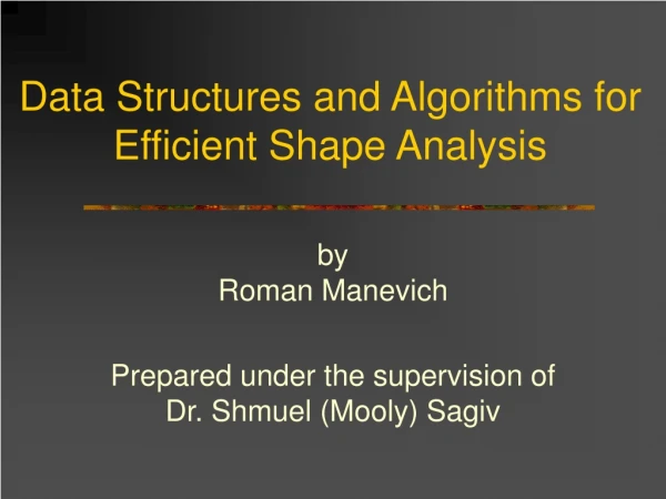
Data Structures and Algorithms for Efficient Shape Analysis

1. Data Structures and Algorithms for Efficient Shape Analysis byRoman Manevich Prepared under the supervision of Dr. Shmuel (Mooly) Sagiv

2. Motivation • TVLA is a powerful and general abstract interpretation system • Abstract interpretation in TVLA • Operational semantics is expressed with first-order logic + TC formulae • Program states are represented assets of Evolving First-Order Structures • Efficiency is an issue

3. Outline • Shape Analysis quick intro • Compactly representing structures • Tuning abstraction to improve performance

4. What is Shape Analysis • Determines Shape Invariants for imperative programs • Can be used to verify a wide range of properties over different programming languages

5. reverse Example /* list.h */typedef struct node { struct node * n; int data;} * List; /* print.c */#include “list.h”List reverse (List x) { List y, t; y = NULL; while (x != NULL) { t = y; y = x; x = xn; yn = t; } return y; }

6. reverse Example Shape before x n . . . n Shape after y n . . . n

7. Definition of a First-Order Logical Structure S = <U, > U – a set of individuals (“node set”)  – a mapping p(r)  (Ur  {0,1}) the “interpretation” of p

8. Information order Three-Valued Logic • 1: True • 0: False • 1/2: Unknown • A join semi-lattice: 0  1 = 1/2 1/2  

9. Canonical Abstraction • Partition the individuals into equivalence classes based on the values of their unary predicates • Collapse other predicates via  • pS(u’1, ..., u’k) =  {pB(u1, ..., uk) | f(u1)=u’1, ..., f(u’k)=u’k) } • At most 3n abstract individuals

10. u0 r[n,x] u0 r[n,x] u r[n,x] Canonical Abstraction Example u1 r[n,x] u2 r[n,x] u3 r[n,x] n n n x n x n

11. Compactly Representing First-Order Logical Structures • Space is a major bottleneck • Analysis explores many logical structures • Reduce space by sharing information across structures

12. Desired Properties • Sparse data structures • Share common sub-structures • Inherited sharing • Incidental sharing due to program invariants • But feasible time performance • Phase sensitive data structures

13. Chapter Outline • Background • First-order structure representations • Base representation (TVLA 0.91) • BDD representation • Empirical evaluation • Conclusion

14. First-Order Logical Structures • Generalize shape graphs • Arbitrary set of individuals • Arbitrary set of predicates on individuals • Dynamically evolving • Usually small changes • Properties are extracted by evaluating first order formula: ∃v1 , v: x(v1) ∧ n(v1, v) • Join operator requires isomorphism testing

15. First-Order Structure ADT • Structure : new() /* empty structure */ • SetOfNodes : nodeSet(Structure) • Node : newNode(Structure) • removeNode(Structure, node) • Kleeneeval(Structure, p(r), <u1, . . . ,ur>) • update(Structure, p(r), <u1, . . . ,ur>, Kleene) • Structurecopy(Structure)

16. print_all Example /* list.h */typedef struct node { struct node * n; int data;} * L; /* print.c */#include “list.h”void print_all(L y) { L x;x = y; while (x != NULL) { /* assert(x != NULL) */ printf(“elem=%d”, xdata);x = xn; }}

17. print_all Example n=½ usm=½ u1y=1 n=½ S1 n=½ usm=½ u1y=1 n=½ S0 x = y x’(v) := y(v) copy(S0) : S1 nodeset(S0) : {u1, u} eval(S0, y, u1) : 1 update(S1, x, u1, 1) x=1 eval(S0, y, u) : 0 update(S1, x, u, 0)

18. print_all Example n=½ while (x != NULL)precondition : ∃v x(v) u1x=1y=1 usm=½ n=½ S1 n=½ x = x  nfocus : ∃v1 x(v1) ∧ n(v1, v)x’(v) := ∃v1 x(v1) ∧ n(v1, v) usm=½ u1y=1 S2.0 n=½ u1y=1 ux=1 S2.1 n=1 n=½ n=½ n=½ u.0sm=½ u1y=1 n=1 S2.2 u.1x=1

19. Overview and Main Results • Two novel representations of first-order structures • New BDD representation • New representation using functional maps • Implementation techniques • Empirical evaluation • Comparison of different representations • Space is reduced by a factor of 4–10 • New representations scale better

20. Base Representation (Tal Lev-Ami SAS 2000) • Two-Level Map : Predicate  (Node Tuple  Kleene) • Sparse Representation • Limited inherited sharing by “Copy-On-Write”

21. BDDs in a Nutshell (Bryant 86) • Ordered Binary Decision Diagrams • Data structure for Boolean functions • Functions are represented as (unique) DAGs x1 x2 x2 x3 x3 x3 x3 0 0 0 1 0 1 0 1

22. BDDs in a Nutshell (Bryant 86) • Ordered Binary Decision Diagrams • Data structure for Boolean functions • Functions are represented as (unique) DAGs • Also achieve sharing across functions x1 x1 x1 x2 x2 x2 x2 x2 x3 x3 x3 x3 x3 x3 x3 0 1 0 1 0 1 Duplicate Terminals Duplicate Nonterminals Redundant Tests

23. Encoding Structures Using Integers • Static encoding of • Predicates • Kleene values • Dynamic encoding of nodes • 0, 1, …, n-1 • Encode predicate p’s values as • ep(p).en(u1). en(u2) . … . en(un) . ek(Kleene)

24. x1 x2 x2 x3 0 1 BDD Representation of Integer Sets • Characteristic function • S={1,5} 1=<001>5=<101> S = (¬x1¬x2x3) (x1¬x2x3)

25. x1 x2 x2 x3 1 BDD Representation of Integer Sets • Characteristic function • S={1,5} 1=<001>5=<101> S = (¬x1¬x2x3) (x1¬x2x3)

26. BDD Representation Example n=½ usm=½ S0 n=½ S0 u1y=1 1

27. BDD Representation Example n=½ usm=½ S0 S1 n=½ S0 u1y=1 x=y n=½ u1x=1y=1 usm=½ n=½ S1 1

28. BDD Representation Example S2.2 n=½ usm=½ S0 S1 n=½ S0 u1y=1 x=y n=½ u1x=1y=1 usm=½ n=½ S1 x=xn n=½ n=½ n=½ u.0sm=½ u1y=1 n=1 S2.2 u.1x=1 1

29. BDD Representation Example S2.2 n=½ usm=½ S0 S1 n=½ S0 u1y=1 x=y n=½ u1x=1y=1 usm=½ n=½ S1 x=xn n=½ n=½ n=½ u.0sm=½ u1y=1 n=1 S2.2 u.1x=1 1

30. Improved BDD Representation • Using this representation directlydoesn’t save space – canonicity doesn’t carry over from propositional to first-order logic • Observation • Node names can be arbitrarily remapped without affecting the ADT semantics • Our heuristics • Use canonic node names to encode nodes and obtain a canonic representation • Increases incidental sharing • Reduces isomorphism test to pointer comparison • 4-10 space reduction

31. Reducing Time Overhead • Current implementation not optimized • Expensive formula evaluation • Hybrid representation • Distinguish between phases:mutable phase  Join  immutable phase • Dynamically switch representations

32. Functional Representation • Alternative representation for first-order structures • Structures represented by maps from integers to Kleene values • Tailored for representing first-order structures • Achieves better results than BDDs • Techniques similar to the BDD representation • More details in the thesis

33. Empirical Evaluation • Benchmarks: • Cleanness Analysis (SAS 2000) • Garbage Collector • CMP (PLDI 2002) of Java Front-End and Kernel Benchmarks • Mobile Ambients (ESOP 2000) • Stress testing the representations • We use “relational analysis” • Save structures in every CFG location

34. Space Results

35. Abstract Counters • Ignore language/implementation details • A more reliable measurement technique • Count only crucial space information • Independent of C/Java

36. Abstract Counters Results

37. Trends in theCleanness Analysis Benchmark

38. Conclusions • Two novel representations of first-order structures • New BDD representation • New representation using functional maps • Implementation techniques • Substantially better than inherited sharing • Structure canonization is crucial • Normalization via hash-consing is the key technique

39. Conclusions • The use of BDDs for static analysis is not a panacea for space saving • Domain-specific encoding crucial for saving space • Failed attempts • Original implementation of Veith’s encoding • PAG

40. Tuning Abstraction for Improved Performance • Analysis can be very costly • Explores many structuresGC example explores >180,000 structures

41. Existing Analysis Modes • Relational analysis • Doubly-exponential in worst case • Our most precise method • Single-structure analysis (Tal Lev-Ami SAS 2000) • Singly-exponential in worst case • Can be very efficient • Can be very imprecise • Sometimes very inefficient

42. Single-Structure Analysis May exist n u1 u x S0 n u1 u x S0  S1 u1 x S1

43. Single-Structure Analysis • Active property • ac=0 doesn’t exist in every concrete structure • ac=1 exists in every concrete structure • ac=1/2 may exist in some concrete structure u1ac=1 n uac=1 x S0 u1ac=1 n uac=1/2 x S0  S1 u1 ac=1 x S1

44. Single-Structure Analysis • Sometimes overly imprecise • Refine analysis by using nullary predicates to distinguish between different structures

45. Is there a “sweet spot”? Efficiency Relational Analysis Precision

46. Chapter Outline • Removing embedded structures • Merging structures with same set of canonical names • Staged analysis to localize abstraction • Merging pseudo-embedded structures

47. Order Relations on Structures and Sets of Structures • S, S’  3-STRUCTSƒS’ if for every predicate p • ps(u1,…,uk)  ps’(ƒ(u1),…, ƒ(uk)) • ({u | ƒ(u)=u’} > 1) sms’(u’) • X, X’  23-STRUCTX  X’ Every SX has S’X’ and SS’

48. Compacting Transformations We look for transformation T: 23-STRUCT 23-STRUCT with the following properties: • Compacting – |T(x)|  |x| • Conservative –T(x)  x Without sacrificing precision

49. u2 r[n,t]r[n,y] u0 r[n,x] u0 r[n,x] u2 r[n,t]r[n,y] ƒ u1 r[n,t]r[n,y] ƒ ƒ Removing Embedded Structures S1 S0 x x n y y u1 r[n,t]r[n,y] n n t t

50. u2 r[n,t]r[n,y] u2 r[n,t]r[n,y] u0 r[n,x] u0 r[n,x] u1 r[n,t]r[n,y] Removing Embedded Structures Reversing a listwith exactly 3 cells Reversing a listwith at least 3 cells S1 S0 x x n y y u1 r[n,t]r[n,y] n n t t