Exploring Elliptic Flow Fluctuations with PHOBOS: A Methodological Study
310 likes | 351 Vues
This study delves into the investigation of elliptic flow fluctuations using the PHOBOS detector. By analyzing the fluctuations in the initial collision region, the Participant Eccentricity Model is tested. The study focuses on measuring v2 fluctuations through different analytical methods, event by event, to validate the model's predictions. The talk outlines the measurement process, ongoing analysis, and simulation experiments conducted at 200 GeV Au-Au collisions. The study also presents a simplified methodological overview of calculating relative abundances of v2 values in samples, emphasizing the extraction of true v2 distributions from observational data.

Exploring Elliptic Flow Fluctuations with PHOBOS: A Methodological Study
E N D
Presentation Transcript
Elliptic Flow Fluctuationswith the PHOBOS detector Burak Alver Massachusetts Institute of Technology
PHOBOS Collaboration Burak Alver, Birger Back,Mark Baker, Maarten Ballintijn, Donald Barton, Russell Betts, Richard Bindel, Wit Busza (Spokesperson), Zhengwei Chai, Vasundhara Chetluru, Edmundo García, Tomasz Gburek, Kristjan Gulbrandsen, Clive Halliwell, Joshua Hamblen, Ian Harnarine, Conor Henderson, David Hofman, Richard Hollis, Roman Holynski, Burt Holzman, Aneta Iordanova, Jay Kane,Piotr Kulinich, Chia Ming Kuo, Wei Li, Willis Lin, Constantin Loizides, Steven Manly, Alice Mignerey, Gerrit van Nieuwenhuizen, Rachid Nouicer, Andrzej Olszewski, Robert Pak, Corey Reed, Eric Richardson, Christof Roland, Gunther Roland, Joe Sagerer, Iouri Sedykh, Chadd Smith, Maciej Stankiewicz, Peter Steinberg, George Stephans, Andrei Sukhanov, Artur Szostak, Marguerite Belt Tonjes, Adam Trzupek, Sergei Vaurynovich, Robin Verdier, Gábor Veres, Peter Walters, Edward Wenger, Donald Willhelm, Frank Wolfs, Barbara Wosiek, Krzysztof Wozniak, Shaun Wyngaardt, Bolek Wyslouch ARGONNE NATIONAL LABORATORY BROOKHAVEN NATIONAL LABORATORY INSTITUTE OF NUCLEAR PHYSICS PAN, KRAKOW MASSACHUSETTS INSTITUTE OF TECHNOLOGY NATIONAL CENTRAL UNIVERSITY, TAIWAN UNIVERSITY OF ILLINOIS AT CHICAGO UNIVERSITY OF MARYLAND UNIVERSITY OF ROCHESTER
Motivation High v2 observed in CuCu can be explained by fluctuations in initial collision region. Can we test the Participant Eccentricity Model?
Au+Au Expected fluctuations Assuming v2part, participant eccentricity model predicts v2 fluctuations Expected v2 from fluctuations in part Data MC
Measuring v2 Fluctuations • We have considered 3 different methods • 2 particle correlations <v22> • c.f. S. Voloshin nucl-th/0606022 • v22= <v22> - <v2>2 • Do systematic errors cancel? • 2 particle correlations v22 event by event • Mixed event background generation is possible • Reduces fit parameters to 1 (no reaction plane) • Hard to untangle acceptance effects event by event • v2 event by event • This is the method we are pursuing
Measuring v2 Fluctuations - Today’s Talk • Measuring v2 event by event • Ongoing analysis on 200GeV Au-Au • Today • How we are planning to make the measurement • Studies on fully simulated MC events • Modified Hijing - Flow • Geant
Method Overview - Simplified Example 2 possible v2 values Event by Event measurement Demonstration Demonstration u=v2obs. Kb(u) Ka(u) or u = v22obs. or u = qobs. V2b V2a V2a V2b Relative abundance in sample Observed u distribution in a sample f1 Demonstration Demonstration g(u) f2 Question: What is the relative abundance of 2 v2’s in the sample?
Method Overview - Simplified Example 2 possible v2 values Event by Event measurement Demonstration Demonstration u=v2obs. Kb(u) Ka(u) or u = v22obs. or u = qobs. V2b V2a V2a V2b Relative abundance in sample Measured u distribution in a sample f1 Demonstration Demonstration g(u) f2 Question: What is the relative abundance of v2a to v2b in the sample?
Method Overview - Simplified Example 2 possible v2 values Event by Event measurement Demonstration Demonstration u=v2obs. Kb(u) Ka(u) or u = v22obs. or u = qobs. V2b V2a V2a V2b Extracted v2true distribution from sample Measured u distribution in a sample fa Demonstration Demonstration g(u) fb V2a V2b Question: What is the relative abundance of v2a to v2b in the sample? g(u)=faKa(u) + fbKb(u)
200 GeV AuAu 200 GeV AuAu Modified Hijing+Geant Modified Hijing+Geant Method Overview Kernel In real life v2 can take a continuum of values u=v2obs. K(u,v2) Extracted v2true distribution from sample Measured u distribution in a sample f(v2) g(u)
Method Overview • 3 Tasks • Measure u event-by-event g(u) • Calculate the kernel K(u,v2) • Extract dynamical fluctuations f(v2)
Hit Distribution PHOBOS Detector • PHOBOS Multiplicity Array -5.4<<5.4 coverage -Holes / granularity differences • Idea: Use all available information in event to read off single u value HIJING + Geant 15-20% central dN/d Primary particles Hits on detector
Measuring u=v2obs Event by Event I • Probability Distribution Function (PDF) for hit positions: Probability of hit in Probability of hit in PDF u demonstration • Define likelihood of u and 0 for an event:
Measuring u=v2obs Event by Event II • Maximize likelihood to find “most likely” value of u • Comparing values of u and 0 • In an event, p(i) is same for all u and 0. • PDF folded by acceptance must be normalized to the same value for different u and 0’s Acceptance
Measuring u=v2obs Event by Event II • Maximize likelihood to find “most likely” value of u • Comparing values of u and 0 • In an event, p(i) is same for all u and 0. • PDF folded by acceptance must be normalized to the same value for different u and 0’s Acceptance
g(u) 200 GeV AuAu Modified Hijing+Geant Measuring u=v2obs Event by Event III Observed u distribution in a sample Mean and RMS of u in slices of v2 Error bars show RMS 200 GeV AuAu Modified Hijing+Geant Next Step: Construct the Kernel to unfold g(u)
200 GeV AuAu Modified Hijing+Geant Calculating the Kernel I • Simple: Measure u distribution in bins of v2 • 2 small complications • Kernel depends on multiplicity: K(u,v2,n) • n = number of hits on the detector • Measure u distribution in bins of v2 and n. • Statistics in bins can be combined by fitting smooth functions
200 GeV AuAu Modified Hijing+Geant Calculating the Kernel II • In a single bin of v2 and n u distribution with for fixed v2 and n (a, b) (<u>,u) • Distribution is not Gaussian • But can be parameterized by <u> and u
200 GeV AuAu 200 GeV AuAu Modified Hijing+Geant Modified Hijing+Geant Calculating the Kernel III • Measure <u> and u in bins of v2 and n • Fit smooth functions K(u,v2,n) K(u,v2,n)
200 GeV AuAu 200 GeV AuAu Modified Hijing+Geant Modified Hijing+Geant Calculating the Kernel IV • Multiplicity dependence can be integrated out K(u,v2 ,n) K(u,v2) N(n) = Number hits distribution in sample
known ? Extracting dynamical fluctuations
Ansatz with two parameters: known ? Extracting dynamical fluctuations Ansatz for f(v2) ansatz Ansatz
Ansatz with two parameters: known ? 200 GeV AuAu Modified Hijing+Geant Extracting dynamical fluctuations Ansatz for f(v2) Expected g(u) for Ansatz ansatz Ansatz integrate
Ansatz with two parameters: known ? 200 GeV AuAu Modified Hijing+Geant Extracting dynamical fluctuations Ansätze for f(v2) Expected g(u) for Ansätze ansatz integrate
Ansatz with two parameters: known ? 200 GeV AuAu Modified Hijing+Geant Extracting dynamical fluctuations Ansätze for f(v2) Comparison with sample ansatz integrate Compare expected g(u) for Ansatz with measurement Minimum 2 <v2> and v2
Method Summary K(u,v2 ,n) MC MC Many MC events integration N(n) K(u,v2) MC MC A Small Sample measurement fin(v2) Minimize 2 in integral <v2>=0.05 v2 =0.02 MC MC <v2>=0.048 v2 = 0.023 measurement g(u) fout(v2)
Verification • Ran this analysis on Modified Hijing • v2() = v2(0) • (1-||/6) • Same as the assumption in our fit • v2(0) given by a Gaussian distribution in each sample • Same as our Ansatz • Analysis done in 10 collision vertex bins • Final results are averaged • 0-40% central events used to construct Kernel • 15-20% central events used as sample
0.04 0.04 0.04 0.02 0.02 0.02 0.02 0.02 0.02 in in in 0.04 0.04 0.04 Verification <v2> = 0.020 • Ran this analysis on Modified Hijing • The input fluctuations are reconstructed successfully out <v2> = 0.050 <v2> = 0.030 200 GeV AuAu 15-20% central out Modified Hijing+Geant <v2> = 0.040 Only statistical errors shown (from combining vertex bins) out
Conclusion / Outlook • A new method to measure elliptic flow fluctuations is developed. • Fluctuations in MC simulations are successfully reconstructed. • Ready to apply the method to extract dynamical fluctuations in DATA. • Important part will be to estimate systematic uncertainties due to the MC/DATA differences • dN/d() • v2() • Non-flow in data • Should show up in reaction plane resolutions
Likelihood Fit Normalization Acceptance
Calculating the Kernel. Functions observed to fit the Kernel