The Two-Factor Mixed Model
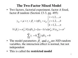
The Two-Factor Mixed Model. Two factors, factorial experiment, factor A fixed, factor B random (Section 13-3, pg. 495) The model parameters are NID random variables, the interaction effect is normal, but not independent This is called the restricted model.

The Two-Factor Mixed Model
E N D
Presentation Transcript
The Two-Factor Mixed Model • Two factors, factorial experiment, factor A fixed, factor B random (Section 13-3, pg. 495) • The model parameters are NID random variables, the interaction effect is normal, but not independent • This is called the restricted model
Testing Hypotheses - Mixed Model • Once again, the standard ANOVA partition is appropriate • Relevant hypotheses: • Test statistics depend on the expectedmeansquares: Ho is rejected if Fo > Fa,a-1,(a-1)(b-1) Fo > Fa,b-1,ab(n-1) Fo > Fa ,(a-1)(b-1), ab(n-1)
Estimating the Variance Components – Two Factor Mixed model • Use the ANOVA method; equate expected mean squares to their observed values: • Estimate the fixed effects (treatment means) as usual
Example 13-3 (pg. 497) The Measurement Systems Capability Study Revisited • Same experimental setting as in example 13-2 • Parts are a random factor, but Operators are fixed • Assume the restricted form of the mixed model • Minitab can analyze the mixed model • The variance components can also be estimated as
Example 13-3 (pg. 497) Minitab Solution – Balanced ANOVA Source DF SS MS F P Part 19 1185.425 62.391 62.92 0.000 Operator 2 2.617 1.308 1.84 0.173 Part*Operator 38 27.050 0.712 0.72 0.861 Error 60 59.500 0.992 Total 119 1274.592 Source Variance Error Expected Mean Square for Each Term component term (using restricted model) 1 Part 10.2332 4 (4) + 6(1) 2 Operator 3 (4) + 2(3) + 40Q[2] 3 Part*Operator -0.1399 4 (4) + 2(3) 4 Error 0.9917 (4)
Example 13-3 Minitab Solution – Balanced ANOVA • There is a large effect of parts (not unexpected) • Small operator effect • No Part – Operator interaction • Negative estimate of the Part – Operator interaction variance component • Fit a reduced model with the Part – Operator interaction deleted • This leads to the same solution that we found previously for the two-factor random model
The Unrestricted Mixed Model • Two factors, factorial experiment, factor A fixed, factor B random (pg. 498) • The random model parameters are now all assumed to be NID . is no longer assumed – unrestricted model
Testing Hypotheses – Unrestricted Mixed Model • The standard ANOVA partition is appropriate • Relevant hypotheses: • Expectedmeansquares determine the test statistics:
Estimating the Variance Components – Unrestricted Mixed Model • Use the ANOVA method; equate expected mean squares to their observed values: • The only change compared to the restricted mixed model is in the estimate of the random effect variance component • Which model to use? • They are fairly close in many cases • The restricted model is slightly more general • The restricted model is mostly preferred
Example 13-4 (pg. 499) Minitab Solution – Unrestricted Model Source DF SS MS F P Part 19 1185.425 62.391 87.65 0.000 Operator 2 2.617 1.308 1.84 0.173 Part*Operator 38 27.050 0.712 0.72 0.861 Error 60 59.500 0.992 Total 119 1274.592 Source Variance Error Expected Mean Square for Each Term component term (using unrestricted model) 1 Part 10.2798 3 (4) + 2(3) + 6(1) 2 Operator 3 (4) + 2(3) + Q[2] 3 Part*Operator -0.1399 4 (4) + 2(3) 4 Error 0.9917 (4)
Sample Size Determination with Random Effects • Consider a single-factor random effects model • Power = 1 – b =P(Reject HoHo is false) • =P(Fo > Fa,a-1,N-aHo is false) • Fo = MSTreatments/MSE (dofs are needed to determine the OC curve) • The operating characteristic curves (Chart VI, Appendix) can be used • The curves plot the probability of type II error against the parameter l
Sample Size Determination with Random Effects – Example 13-5 • Five treatments randomly selected (a = 5) • Six observations per treatment (n = 6) • a = 0.05, a – 1 = 4 (v1), N – a = 25 (v2) • Assume that • Then • b 0.20
Sample Size Determination with Random Effects • Use the percentage increase in the standard deviation of an observation • If the treatments are homogeneous, s • If the treatments are different, • P is the fixed percentage increase in the standard deviation • Then
Sample Size Determination with Random Effects – Two Factors Table 13-8
Finding Expected Mean Squares • Obviously important in determining the form of the test statistic • In fixed models, it’s easy: • Can always use the “brute force” approach – just apply the expectation operator • Straightforward but tedious • Rules on page 502-503 [due to Cornfield and Tukey (1956)] work for any balanced model • Rules are consistent with the restricted mixed model
Approximate F Tests • Sometimes we find that there are no exact tests for certain effects
Approximate F Tests • One possibility: assume that certain interactions are negligible – needs conclusive evidence • If we cannot assume that certain interactions are negligible, then use an approximate F test (“pseudo” F test) • Test procedure is due to Satterthwaite (1946), and uses linearcombinations of the original mean squares to form the F-ratio • For example: • MS’ = MSr + …+ MSs • MS’’ = MSu + …+ MSv • The mean squares are chosen so that E(MS’) – E(MS’’) is a multiple of the effect considered in the null hypothesis • F is distributed approximately as Fp,q
Approximate F Tests • The linear combinations of the original mean squares are sometimes called “synthetic” mean squares • Adjustments are required to the degrees of freedom • Refer to Example 13-7, page 505 • Minitab will analyze these experiments, although their “synthetic” mean squares are not always the best choice