Download
1 / 29
310 likes | 711 Vues
PVT Behavior of Fluids and the Theorem of Corresponding States. Compressibility Factor The volumetric PVT behavior of a material is often characterized by the compressibility factor Z Typical values: ideal gas, Z = 1.0; liquids, Z ~ 0.01 to 0.2; critical point, Z c ~ 0.27 to 0.29

E N D
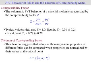
PVT Behavior of Fluids and the Theorem of Corresponding States • Compressibility Factor • The volumetric PVT behavior of a material is often characterized by the compressibility factor Z • Typical values: ideal gas, Z = 1.0; liquids, Z ~ 0.01 to 0.2; critical point, Zc ~ 0.27 to 0.29 • Theorem of Corresponding States • This theorem suggests that values of thermodynamic properties of different fluids can be compared when properties are normalized by their values at the critical point
PVT Behavior of Fluids and the Theorem of Corresponding States • Theorem of Corresponding States • The reduced temperature and pressure are simply • If Zc is assumed to be a constant for all materials • Experimental observationsprovide strong evidence to support this approach • The relation above indicates that all fluids have the same reduced volume Vr (as well as other properties) at a specified Tr and Pr • In Example 7.2 the principle of corresponding states was used to relate the a and b constants of the van der Waals equation of state to a fluids critical properties, specifically Tc and Pc and
PVT Behavior of Fluids and the Theorem of Corresponding States • Generalized Coexistence Curve • The theorem of corresponding states can be used to obtain a generalized phase diagram • “Law of rectilinear diameters” – states that the average density in the L-V region varies linearly over a wide temperature range below the critical point • Zeno line – the Z = 1.0 line on the phase diagram • For states with Z > 1.0 (hard fluid), repulsive forces dominate and conversely, for states where Z < 1.0 (soft fluid) attractive forces are dominant
PVT Behavior of Fluids and the Theorem of Corresponding States • Acentric Factor • To improve the accuracy of property predictions, Pitzer and coworkers introduced the acentric factor w as a third correlating parameter • The acentric factor was developed as a measure of the difference in structure between the material of interest and a spherically symmetric gas such as argon • Therefore, the parameter is related to a molecular property • The parameter is defined using the reduced vapor pressure
PVTN Equations of State for Fluids • Overview • Although the corresponding states correlations are useful, the data is displayed in charts and graphs are therefore cumbersome to use • A more useful means to express a fluids PVT behavior is through an analytical expression (PVT equation of state) • Two general approaches • Statistical mechanical models – based on rigorous theoretical principles accounting for the interactions between molecules (preferred by physicists and physical chemists) • Empirical expressions – models formulated by determining parameters in a mathematical expression through a fit to experimental data (preferred by chemical engineers)
PVTN Equations of State for Fluids • Relating EOS Parameters to Experimental Data • Empirical models have parameters that must be determined to calculate PVT data • A common way to determine these parameters is to relate the model parameters to a fluid’s critical properties • By adopting this approach we are utilizing the theorem of corresponding states • The critical point criteria for a single-component system require • Recall Example 7.2, where these criteria were used to determine the parameters for the van der Waals EOS and
PVTN Equations of State for Fluids • Cubic Equations of State • Since the pioneering work of van der Waals, numerous modifications of the original vdW EOS have been published • Most are pressure-explicit cubic forms, i.e., • van der Waals EOS and Zc = 0.375
PVTN Equations of State for Fluids Redlich-Kwong Zc = 0.333 with with • Redlich-Kwong-Soave • The attractive term is made temperature dependent and the acentric factor is introduced • with Zc = 0.333
PVTN Equations of State for Fluids Peng-Robinson Zc = 0.307 with
PVTN Equations of State for Fluids • Hard-Sphere Equation of State • A class of EOSs that incorporate knowledge of the specific molecular interactions with additional fitted parameters • The repulsive term is theoretically based • The term bo below accounts for the excluded volume of a molecule • The attractive term is empirical • Here is one example of a hard-sphere EOS that uses the Carnahan-Starling repulsive term and van der Waals attractive term s→ molecular diameter
PVTN Equations of State for Fluids • Virial-Type Equation of State • An important EOS class that has a rigorous basis in molecular theory (may be derived from statistical mechanics) • The compressibility is expressed as a polynomial in volume • Or as a polynomial expansion in pressure • Where • The coefficients B, C, D, … are termed the second, third, fourth, … virial coefficients
PVTN Equations of State for Fluids • Method of Abbott • The virial equation is truncated after the second virial coefficient term and the pressure is obtained • The second virial coefficient is expressed in terms of two functions of temperature B(0) and B(1) as well as the acentric factor • Where and
PVTN Equations of State for Fluids • Benedict-Webb-Rubin EOS • Another example of a virial-type EOS • Has eight parameters • Frequently used for modeling the PVT behavior of light hydrocarbons and gases in petroleum and natural gas applications
Evaluating Changes in Properties Using Departure Functions • Overview • We now develop methods for determining changes in derived thermodynamic properties of a pure substance • Because properties are state functions, we can choose any convenient path to calculate the change in the property of interest (e.g., H, S, U, A, or G) • To perform the calculation, we must generally have access to two constitutive relationships • A PVT or PVTN equation of state (EOS) • An ideal-gas state heat capacity equation
Evaluating Changes in Properties Using Departure Functions • Convenient Path • To calculate property changes between two well-defined states (T1,P1,V1) and (T2,P2,V2) we use the following three-step process • Isothermal expansion at T1 from P = P1 to 0 (or V = V1 to ∞ • Isobaric (or isochoric) heating from T1 to T2 in an attenuated ideal gas state [P = 0 (or V = ∞)] • Isothermal compression at T2 from P = 0 to P2(or from V = ∞ to V2)
Evaluating Changes in Properties Using Departure Functions • Convenient Path • The total property change between states 1 and 2, DB (where B is one of H, S, U, A, or G), is the sum over these three steps • Step (2) occurs entirely within the ideal-gas state • Recall that only 2 of the 3 intensive variables T, P, and V are independent • We select T as one independent variable and choose P or V based on the PVT EOS we have • If we have a pressure-explicit EOS (P = f (T,V)), we choose V • If we have a volume-explicit EOS (V = f (T,P)), we choose P step (1) step (2) step (3)
Evaluating Changes in Properties Using Departure Functions • Example 8.3 • Develop expressions for DS between states 1 and 2 assuming you have analytic forms for (1) a volume-explicit EOS and (2) a pressure-explicit EOS and • Summary Volume-explicit EOS Pressure-explicit EOS
Evaluating Changes in Properties Using Departure Functions • Departure (Residual) Functions • A departure function is the difference between the property of interest in its real state at a specified T, P, and V and in an ideal-gas state at the same temperature T and pressure P • There are two equivalent forms of the departure function • B is any derived property (H, S, U, A, or G) and Vo = RT / P(T,V)
Evaluating Changes in Properties Using Departure Functions • Residual Entropy • Based on Example 8.3, the residual entropy is defined as
Evaluating Changes in Properties Using Departure Functions • Residual Helmholtz Energy • When working with pressure-explicit EOSs, the departure function for the Hemlholtz energy is particularly useful • The differential expression for A is • Integrating at constant T between A(T,V) and A(T,∞) gives • To obtain the departure function, we must also account for the change from V→ ∞ to V = Vo, which occurs in the ideal-gas state • To avoid a singularity we also add and subtract
Evaluating Changes in Properties Using Departure Functions • Residual Helmholtz Energy • The final result is • Residual Entropy • The entropy is obtained by differentiating A with respect to T
Evaluating Changes in Properties Using Departure Functions • Other Departure Functions • Now that A and S are known, other departure functions can be obtained through simple algebra • General Result • To determine the change in a thermodynamic property between two states, we evaluate two isothermal departure functions (at T1 and T2) and a temperature change contribution in the ideal gas state departure function at T1 departure function at T2 ideal-gas isotherm
Evaluating Changes in Properties Using Departure Functions • Departure Functions for Volume-Explicit PVT EOSs • When volume-explicit PVT EOSs are available the following isothermal departure functions should be used
Evaluating Changes in Properties Using Departure Functions Useful Ideal-Gas Property Relationships Internal Energy: Enthalpy: Entropy:
Evaluating Changes in Properties Using Departure Functions • Heat Capacity Departure Functions (Pressure-Explicit PVT EOS) • The heat capacities are related to differentials of the entropy with temperature, for example Cv is defined as • Evaluating the derivative yields • The constant pressure heat capacity departure function requires a bit more work to obtain • Often times it is more convenient to obtain Cp – Cpo by first determining Cv – Cvo and then using an expression that relates Cv and Cp that will be introduced below
Evaluating Changes in Properties Using Departure Functions • Heat Capacity Departure Functions (Volume-Explicit PVT EOS) • With a volume-explicit PVT EOS the constant pressure heat capacity departure function is relatively straightforward to obtain • Evaluating the derivative yields
Evaluating Changes in Properties Using Departure Functions • General Relationships Between Cv and Cp • Using the formalism introduced in Chapter 5 one can obtain the following relationship between Cv and Cp • The above expression is completely general and therefore can be used to relate heat capacities for real or ideal gases as well as for liquids and solids • Recalling the definitions of kT and ap, the expression above can equivalently be written as
Compressibility and Heat Capacity of Solids • Incompressible Substances • Most solids and many liquids far below their critical temperatures have very low compressibilities • In these situations one can assume perfectly or nearly incompressible behavior as a first-order approximation • An incompressible substance is defined as having a constant volume (V= constant) independent of T and P • From this definition, it follows that ap = kT = 0 for an incompressible substance • For a nearly incompressible substance the following expressions are appropriate (for a perfectly incompressible substance, the approximation becomes a true equality)
Derived Property Representations • Overview • Before the infusion of computers, charts or tubular data were used widely for engineering problem solving • Although computer-generated representations of thermodynamic properties are preferred, many graphical forms of data are still used in engineering practice • The temperature-entropy (T-S) diagram for water is a good example


![[READ DOWNLOAD] Phase Behavior of Petroleum Reservoir Fluids](https://cdn7.slideserve.com/12657129/read-download-phase-behavior-of-petroleum-dt.jpg)