CS 321 Programming Languages and Compilers Lectures 16 & 17
CS 321 Programming Languages and Compilers Lectures 16 & 17. Introduction to Formal Languages Regular Languages Lexical Analysis. Languages. Have a finite vocabulary Have finite length sentences Have possibly infinitely many sentences. Grammars and Recognizers.

CS 321 Programming Languages and Compilers Lectures 16 & 17
E N D
Presentation Transcript
CS 321Programming Languages and CompilersLectures 16 & 17 Introduction to Formal Languages Regular Languages Lexical Analysis
Languages • Have a finite vocabulary • Have finite length sentences • Have possibly infinitely many sentences Finite Automata & Lexing
Grammars and Recognizers • A Grammar is a finitary method by which all sentences of a language, L, may be generated via well-defined rules. • A Recognizer is a procedure which, given a “string” x, answers “yes” if x L • We usually also want to answer “no” if x L, I.e. usually demand an algorithm.) Finite Automata & Lexing
(Context-Free) Grammars • Def. A (context-free or Chomsky Type-2) grammar (cfg) is a 4-tuple G = (N, , P, S) where • N is a finite, non-empty set of symbols (non-terminal vocabulary) • is a finite set of symbols (terminal vocabulary) • N = • V N (vocabulary) • S N (goal symbol) • P is a finite subset of N V* (production rules) Finite Automata & Lexing
Set Operations • Def. Let X and Y be sets of words XY {xy | x X and y Y} X0 {} (where represents the empty string) X1 X XI+1 XiX X* i 0 Xi X+ i > 0 Xi (soX+ =X* X) Finite Automata & Lexing
Example • G = (N, , P, E) where N = {E, T, F} = {[, ], +, *, id} P = {(E,T), (E,E+T), (T,F), (T,T*F), (F,id), (F,[E])} • (so V = N = {E, T, F, [, ], +, *, id}) • (A, ) P is usually written A or A ::= or A : Finite Automata & Lexing
Convention • Given G = (N, , P, S) (with V = N ) (or G = (V, , P, S) with N=V- ) • elements of N: A, B, … • elements of V: … U, V, W, X, Y, Z • elements of : a, b, … • elements of *: … u, v, w, x, y, z • elements of V *: , , , , , • others: • names (not underlined) : N • S: N • underlined or courier font: • special symbols: • is used to denote a production rule: ( = A ) Finite Automata & Lexing
Generating L • How to use a grammar, G, to generate a sentence in L(G): • Begin with a string, consisting of only the goal symbol. • repeat select from a non-terminal “A” and “rewrite” A according to some production (A, ) thereby producing ’ from . until ’ * Finite Automata & Lexing
Example G = (N, , P, S) where P is (abbreviated) as follows: E T | E + T T F | T * F F id | < E > and where N = {E, T, F, Q} = {+, *, <, >, id} S = E Finite Automata & Lexing
Regular Sets • Regular sets (also called regular languages) are defined as follows. Let be a finite alphabet. 1) is a regular set over . 2) {} is a regular set over . 3) a , {a} is a regular set over . 4) If P and Q are regular sets over , a) P Q is a regular set over . b) PQ is a regular set over . c) P* is a regular set over . 5) Nothing else is a regular set over . Finite Automata & Lexing
Regular Expressions 1) denotes the regular set . 2) denotes the regular set {}. 3) a denotes the regular set {a}. 4) If p and q are regular expressions denoting the regular sets P and Q respectively, then a) (p|q) denotes P Q. b) (pq) denotes PQ. c) (p)* denotes p* 5) Nothing else is a regular expression. *** Notation: (p)+ ((p)*p) (p)? p | Finite Automata & Lexing
Right-Linear Grammars (Generators for Regular Sets) • Def. Let G = (N, , P, S) be a cfg. G is said to be right-linear if P N (* *N) *** • Proposition. If G is a right-linear cfg then L(G) is a regular set over . • Proposition. If R is a regular set over , then a right-linear cfg, G, for which L(G) = R. Finite Automata & Lexing
Finite Automata (Recognizers for Regular Sets) Def. A deterministic finite automaton (deterministic finite state machine) is a 5-tuple: M = (Q, , , q0, F) where 1) Q is a finite non-empty set of states. 2) is a finite set of input symbols. 3) q0 Q (initial state) 4) F Q (final states) 5) is a partial mapping from Q to Q (transition function or move function) Finite Automata & Lexing
q 0|1 p 0|1 start 0|1 r s 0|1 Transition Diagrams • FSMs are often visualized as transition diagrams. Finite Automata & Lexing
Finite State Machines • The preceding transition diagram can be represented by a tabular move function: Finite Automata & Lexing
q0 F Q Finite State Machines • The preceding transition diagram can be represented by a tabular move function: Finite Automata & Lexing
Formalizing the Moves of a FSM • A pair (q,u) in Q * is called a configuration of M. • (q0, u) is an initial configuration. • M proceeds from one configuration to the next by moving according to the transition function: (q, au) (q’, u) if (q, a)=q’ (q, u) … (q’, v) is written (q, u) * (q’, v) • The language accepted (or defined) by M is L(M) = {u * | (q0, u) * (q, ) for some q F} Note: Sometimes is used to denote the empty string Finite Automata & Lexing
Example • With the machine M = ({p,q,r,s}, {0,1, }, , p, {q,r}) where the move function is shown in the preceding table. • Question 1: Is 010 L(M)? • Question 2: Is L(M)? • Question 3: Is 010 L(M)? Finite Automata & Lexing
“Complete” Finite State Machines • Extend : Finite Automata & Lexing
0|1 0|1 q start 0|1 p r 0|1 0|1| s t Complete Finite State MachineTransition Diagram Version Finite Automata & Lexing
Non-deterministic FSMs • A FSM may have a choice of moves, i.e. is a mapping from Q to 2Q. • Proposition. Let M1 be a non-deterministic FSM. Then a DFSM M2 for which L(M2) = L(M1). • Proposition. Given a NFSM, M, one can construct a right-linear cfg, G, for which L(G) = L(M), and conversely. Finite Automata & Lexing
Extended Non-determinism • Besides allowing multiple moves on the same input symbol, we can allow moves on the empty string, ; i.e. for a given state q: (q, ) Q Finite Automata & Lexing
start start a|b 3 b b 0 1 2 a a a 2 1 0 b 4 b 3 Examples Finite Automata & Lexing
start i f Thompson’s Construction • Given a regular expression, r representing a regular set R, construct a non-deterministic finite state machine M that recognizes R, i.e. such that L(M)=R. 1) For construct Finite Automata & Lexing
start Thompson’s Construction 2) For a in construct i a f Finite Automata & Lexing
start s f N(s) N(t) Thompson’s Construction 3) Suppose N(s) and N(t) are NFSM's for regular expressions s and t. a) For the regular expression s|t, construct Finite Automata & Lexing
start N(s) N(t) i f Thompson’s Construction b) For the regular expression st, construct: Finite Automata & Lexing
start f i N(s) Thompson’s Construction c) For the regular expression s*, construct Finite Automata & Lexing
Transforming a NFSM to a DFSM (The Subset Construction) • Define: -closure(sQ) = {tQ | s can reach t via only -moves} -closure(T Q) = -closure(s) move(T Q, a ) = (s,a) sT sT Finite Automata & Lexing
NFSM DFSM • Given M=(Q, , , q0, F) define M’=(Q’, , ’, q’0, F’) by: 1) Compute q’0 = -closure(q0). 2) Initialize Q’ with q’0 (unmarked). 3) while an unmarked element q’ of Q’: a) mark q’ b) a : -- compute p’ = -closure(move(q’, a)) -- if p’ Q’ then add p’ (unmarked) to Q’ -- set ’(q’, a)=p’ 4) F’ = { q’ Q’ | q q’ q F} Finite Automata & Lexing
Example • Perform Thompson’s Construction on (a|b)*abb to obtain a non-deterministic finite state machine. • Perform the subset construction to make it deterministic. Finite Automata & Lexing
Simulating a DFSM s:= q0 a:=nextchar while a eof { s:= (s,a) a:=nextchar } if s F thenreturn “yes” elsereturn “no” Finite Automata & Lexing
Simulating a NFSM S:= -closure({q0}) a:=nextchar while a eof { S:= -closure(move(S,a)) a:=nextchar } if S F thenreturn “yes” elsereturn “no” Finite Automata & Lexing
Transforming from NFSM to Right-Linear CFG • Given M=(Q, , , q0, F), construct G=(Q, , P, q0) where 1) q F include in P q 2) q1, q2 Q; a q2 (q1, a) include in P q1 a q2 3) q1, q2 Q q2 (q1, ) include in P q1 q2 Finite Automata & Lexing
start a|b 3 b b 0 1 2 a Example • Let M be: (Note, this is not something obtained from Thompson’s Construction, but written by hand.) • We have: q0 a q0 | b q0 | a q1 q1 b q2 q2 b q3 q3 Finite Automata & Lexing
RLG Regular Expression • The algorithm resembles Gaussian Elimination. • Notice that all of the “A-rules” can be “grouped” by the non-terminal on the right side of the right-part and “factored”: A 0A A 1A1 A 2A2 … A n-1An-1 A n where the iare regular expressions over Finite Automata & Lexing
RLG Regular Expression • Then A can be written as the following regular expression over V: A = 0*( 1A1 | 2A2 | … | n-1An-1 | n ) and the above regular expression can be substituted for A everywhere A appears in the grammar. • Following that, all rules can again be written in the foregoing “factored” form. Finite Automata & Lexing
RLG Regular Expression • Given a right-linear grammar G=(N, . P, S): A) repeat 1) write all rules in “factored” form. 2) choose some non-terminal, A S, to eliminate. 3) compute the regular expression, r, which is equivalent to A, and substitute r in place of A everywhere in G. 4) delete all A-rules from G until only S-rules remain B) compute the regular expression, r, to which S is equivalent. Finite Automata & Lexing
Example • Recall q0 a q0 | b q0 | a q1 q1 b q2 q2 b q3 q3 • Rewrite q0 (a | b) q0 | a q1 q1 b q2 q2 b q3 q3 Finite Automata & Lexing
Example • Eliminate q3 q0 (a | b) q0 | a q1 q1 b q2 q2 b • Eliminate q2 q0 (a | b) q0 | a q1 q1 b b • Eliminate q1 q0 (a | b) q0 | a b b • Compute q0 q0= (a | b)* a b b Finite Automata & Lexing
Limitations of FSMs • FSMs have a fixed numbers of states • For this reason, there are objects that cannot be recognized by FSMs. • For example there is no FSM that can recognize palindromes of arbitrary length. • The DO keyword in Fortran cannot be expressed as a regular expression. Finite Automata & Lexing
Minimization of DFSM’s • Well-known algorithm (due to Hopcroft), useful in many other circumstances. 1) Initially partition Q into two groups, F and Q-F. 2) repeat group, G, of the partition, split G into multiple sub-groups, if incompatible transitions are found among members of G. until no further changes occur Finite Automata & Lexing
Example final Finite Automata & Lexing
Algebraic Properties Finite Automata & Lexing
Shorthand Notations • (a)+ denotes one or more instance r* = r+ | r+ = rr* • (r)? denotes zero or one instance r? = r | • [a-z] denotes a|b|c|..|z Finite Automata & Lexing
Examples • [a-zA-Z]+ denotes string of one or more characters • [a-zA-Z][a-zA-Z0-9] + denotes valid identifiers in Fortran • [0-9] +(.[0-9] +)?(E(+|-)?[0-9] +)? denotes valid unsigned Pascal numbers Finite Automata & Lexing
Extended Transition Diagrams for Parts of Pascal Finite Automata & Lexing