Lab 6: Projectiles

1. Lab 6: Projectiles CS 282

2. Overview • Review of projectile physics • Examine gravity projectile model • Examine drag forces • Simulate drag on a projectile • Examine wind forces • Simulate wind affecting a projectile

3. General Concepts • Acceleration • F = ma • Translational velocity and state • dv/dt = a , ds/dt = v • Rotational acceleration • torque = inertia * rotational_acceleration • Equations of motion are separated into directional components

4. Reference Frame • Let’s use Cartesian Coordinates for simplicity

6. Gravity-Only Projectile Model • Fx = 0 • Fy = -mg • Fz = 0 • vx = vx0 • vy = vy0 –gt • vz=vz0 • ax = 0 • ay = –g • az= 0

7. Exercise 1: Setting Up • Please sit next to your partner (if possible) • Download the framework code for today • Available on the class website • Examine the projectile class • Look at the gravity_model function • !!!! Fill in the missing update y-position !!!! • Compile and run • If necessary, WASD2X translates the camera (use at your own risk though  ) • ENTER toggles the simulation ON/OFF

8. Exercise 1: Setting Up • Hopefully, you have come up with something like (without cheating) this… • position.y + vy *dt+ 0.5*g*dt2 • For this lab, let’s just assume there’s a golf club (or something) is hitting that projectile  • So, Gravity-Only models are… • Really easy to implement • Feasible to analytically solve • Really unrealistic looking

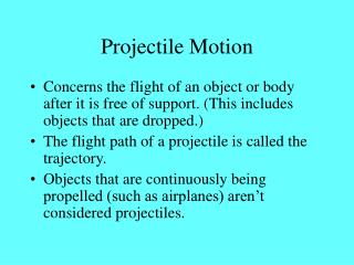
9. Summary: Gravity-only model • The only force on the projectile is gravity • Only acts on the vertical (or the y) direction • The motion in the three directions is independent. • What happens in the y-direction , for example, does not effect the x- or z-directions • The velocity in the x- and z-directions is constant throughout the trajectory • The shape of the trajectory will always be a parabola

10. Let’s Spice Things Up!

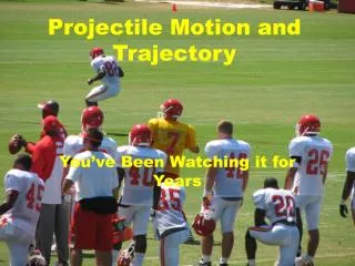
11. Aerodynamic Drag • What is drag? • The resistance that air or any other type of gas exerts on a body traveling through it. • Drag directly resists velocity • X, Y, and Z velocities

12. Drag: Overview • Drag has two components • Pressure drag: Caused by the differences in pressure between the front and back of the object • Skin drag: As the projectile is moving through space, friction is created between it and the gas

13. Drag Coefficient • The drag coefficient, Cd, is a scalar used to evaluate drag force. • The shape of an object greatly affects how much drag affects it.

14. Exercise 2: Implementing Drag • Examine the projectile class • You will notice a function called “drag_model” • This is where you will drag will be implemented • You will also notice several data members in the class that are related to drag. • Part of the drag_model function should look suspiciously familiar. • Indeed, it is our favorite Runge-Kutta method! • Or at least, a fragment of it…

15. Exercise 2: Implementing Drag • The goal for this exercise is to finish the rest of the Runge-Kutta approximation of drag. • The first step of runge-kutta is provided for you • Here are some relevant equations: • Fx = -Fd (vx/v) Fy = -mg -Fd (vy/v) • Fz =- Fd (vz/v) • The force due to drag is • Fd = ½ p *v2 *A *Cd • 0.5 * density * velocity2 * cross-area * drag coeff.

16. Exercise 2: Implementing Drag • First , finish steps 2 through 4 of the Runge-Kuttaprocces • Use step 1 and the equations as a reference • Be careful! Because we have more than one velocity (as opposed to just x-velocity last time), you will have k’s for each component • Don’t forget to average your k’s before you add it to the velocity, and update your position.

17. Summary: Aerodynamic Drag • Drag force acts in the opposite direction to the velocity. The magnitude of the drag force is proportional to the square of the velocity • Drag causes the three components of motion to become coupled (i.ex depends on y and z) • The drag force is a function of the projectile geometry and is proportional to both the frontal area and drag coefficient of the projectile

18. Summary: Drag (end) • The acceleration due to drag is inversely proportional to the mass of the projectile. Other things being equal, a heavier projectile will show fewer drag effects than a lighter projectile. • The drag on an object is proportional to the density of the fluid in which it is traveling.

19. And like Reno’s Weather…

20. Getting Windy? • Now that we have drag, it will be relatively easier to add wind into our simulation. • The presence of wind changes the apparent velocity seen by a projectile • Tail-wind adds to the velocity of the object. • Head-wind subtracts from the velocity

21. Exercise 3: Wind • Luckily for us, since we’ve implemented drag already, it will be easy to add wind. • You may have already noticed a function, as well as parameters, hiding in the projectile class relating to wind. • First of all, let’s keep all the work we did for drag. Go ahead and copy paste the contents of the function into the blank function “drag_wind_model”

22. Exercise 3: Wind • Now, all we have to do is subtract the wind’s velocity components from each section of the Runge-Kutta steps • Tail-winds will have negative velocity, thus increasing our end velocity • The reverse for head-winds

23. That’s all Folks! • Save your finished product somewhere. • Perchance commit it to a repository? • You will be needing this for next week when we add on… • Spin • Different shaped objects • Mystery?

24. (kind of) For next week… • Plot the differences between the following combinations on a graph (position vs. time) • Gravity only • Gravity and drag • Gravity and tail-wind • Gravity, head-wind, and drag • Not due next week, but you will be adding more things to your simulation, so having this done will lesson your workload next week.