Dynamic Programming
Learn how dynamic programming optimizes problem-solving by avoiding redundant calculations through sub-problems. Explore the concept using Fibonacci series as an example.

Dynamic Programming
E N D
Presentation Transcript
Dynamic Programming ITS033 – Programming & Algorithms Topic 07 Asst. Prof. Dr. Bunyarit Uyyanonvara IT Program, Image and Vision Computing Lab. School of Information and Computer Technology Sirindhorn International Institute of Technology Thammasat University http://www.siit.tu.ac.th/bunyaritbunyarit@siit.tu.ac.th02 5013505 X 2005
ITS033 Midterm Topic 01-Problems & Algorithmic Problem Solving Topic 02 – Algorithm Representation & Efficiency Analysis Topic 03 - State Space of a problem Topic 04 - Brute Force Algorithm Topic 05 - Divide and Conquer Topic 06-Decrease and Conquer Topic 07 - Dynamics Programming Topic 08-Transform and Conquer Topic 09 - Graph Algorithms Topic 10 - Minimum Spanning Tree Topic 11 - Shortest Path Problem Topic 12 - Coping with the Limitations of Algorithms Power http://www.siit.tu.ac.th/bunyarit/its033.php and http://www.vcharkarn.com/vlesson/showlesson.php?lessonid=7
This Week Overview • Dynamic Programming • Fibonacci Series • Knapsack Problem • Memory Function
Dynamic Programming: Introduction Topic 07.1 ITS033 – Programming & Algorithms Asst. Prof. Dr. Bunyarit Uyyanonvara IT Program, Image and Vision Computing Lab. School of Information and Computer Technology Sirindhorn International Institute of Technology Thammasat University http://www.siit.tu.ac.th/bunyaritbunyarit@siit.tu.ac.th02 5013505 X 2005
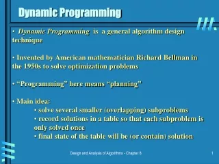
Introduction • Dynamic programming is a technique for solving problems with overlapping sub-problems. • Typically, these sub-problems arise from a recurrence relating a solution to a given problem with solutions to its smaller sub-problems of the same type.
Introduction • Rather than solving overlapping sub-problems again and again, • dynamic programming suggests solving each of the smaller sub-problems only once • and recording the results in a table from which we can then obtain a solution to the original problem.
Introduction • The Fibonacci numbers are the elements of the sequence 0, 1, 1, 2, 3, 5, 8, 13, 21, 34, . . . , Algorithm fib(n) if n = 0 or n = 1 return 1 return fib(n − 1) + fib(n − 2) • The original problem F(n) is defined by F(n-1) and F(n-2)
Introduction • The Fibonacci numbers are the elements of the sequence 0, 1, 1, 2, 3, 5, 8, 13, 21, 34, . . . , Algorithm fib(n) if n = 0 or n = 1 return 1 return fib(n − 1) + fib(n − 2) • If we try to use recurrence directly to compute the nth Fibonacci • number F(n) , we would have to recompute the same values of this function many times • in fact, we can avoid using an extra array to accomplish this task by recording the values of just the last two elements of the Fibonaccisequence
Introduction • Notice that if we call, say, fib(5), we produce a call tree that calls the function on the same value many different times: • fib(5) • fib(4) + fib(3) • (fib(3) + fib(2)) + (fib(2) + fib(1)) • ((fib(2) + fib(1)) + (fib(1) + fib(0))) + ((fib(1) + fib(0)) + fib(1)) • (((fib(1) + fib(0)) + fib(1)) + (fib(1) + fib(0))) + ((fib(1) + fib(0)) + fib(1)) • If we try to use recurrence directly to compute the nth Fibonacci number F(n) , we would have to recompute the same values of this function many times
Introduction • Certain algorithms compute the nth Fibonacci number without computing all the preceding elements of this sequence. • It is typical of an algorithm based on the classic bottom-up dynamic programming approach, • A top-down variation of it exploits so-called memory functions • The crucial step in designing such an algorithm remains the same => Deriving a recurrence relating a solution to the problem’s instance with solutions of its smaller (and overlapping) subinstances.
Introduction • Dynamic programming usually takes one of two approaches: • Bottom-up approach: All subproblems that might be needed are solved in advance and then used to build up solutions to larger problems. This approach is slightly better in stack space and number of function calls, but it is sometimes not intuitive to figure out all the subproblems needed for solving the given problem. • Top-down approach: The problem is broken into subproblems, and these subproblems are solved and the solutions remembered, in case they need to be solved again. This is recursion and Memory Function combined together.
Bottom Up • In the bottom-up approach we calculate the smaller values of Fibo first, then build larger values from them. This method also uses linear (O(n)) time since it contains a loop that repeats n − 1 times. • In both these examples, we only calculate fib(2) one time, and then use it to calculate both fib(4) and fib(3), instead of computing it every time either of them is evaluated. Algorithm Fibo(n) previousFib = 0, currentFib = 1 repeat n − 1 times newFib = previousFib + currentFib previousFib = currentFib currentFib = newFib return currentFib
Top-Down • suppose we have a simple map object, m, which maps each value of Fibo that has already been calculated to its result, and we modify our function to use it and update it. The resulting function requires only O(n) time instead of exponential time: • This technique of saving values that have already been calculated is called Memory Function; this is the top-down approach, since we first break the problem into subproblems and then calculate and store values m [0] = 0 m [1] = 1 Algorithm Fibo(n) if map m does not contain key n m[n] := Fibo(n − 1) + Fibo(n − 2) return m[n]
Dynamic Programming: Knapsack Problem Topic 07.2 ITS033 – Programming & Algorithms Asst. Prof. Dr. Bunyarit Uyyanonvara IT Program, Image and Vision Computing Lab. School of Information and Computer Technology Sirindhorn International Institute of Technology Thammasat University http://www.siit.tu.ac.th/bunyaritbunyarit@siit.tu.ac.th02 5013505 X 2005
0-1 Knapsack problem • Given a knapsack with maximum capacity W, and a set S consisting of n items • Each item i has some weight wi and benefit value bi(all wi , biand W are integer values) • Problem: How to pack the knapsack to achieve maximum total value of packed items?
W = 20 0-1 Knapsack problem: Weight Benefit value bi wi Items 3 2 This is a knapsack Max weight: W = 20 4 3 5 4 8 5 10 9
0-1 Knapsack problem • Problem, in other words, is to find • The problem is called a “0-1” problem, because each item must be entirely accepted or rejected. • Just another version of this problem is the “Fractional Knapsack Problem”, where we can take fractions of items. (see Greedy Algorithm)
0-1 Knapsack problem: brute-force approach • Since there are n items, there are 2n possible combinations of items. • We go through all combinations and find the one with the most total value and with total weight less or equal to W • Running time will be O(2n)
0-1 Knapsack problem • Can we do better? • Yes, with an algorithm based on dynamic programming • We need to carefully identify the subproblems
The Knapsack Problem • To design a dynamic programming algorithm, • we need to derive a recurrence relation that expresses a solution to an instance of the knapsack problem • in terms of solutions to its smaller sub-instances.
Recursive Formula for subproblems • It means, that the best subset of Sk that has total weight w is one of the two: 1) the best subset of Sk-1 that has total weight w, or 2) the best subset of Sk-1 that has total weight w-wk plus the item k • Recursive formula for subproblems:
Recursive Formula • The best subset of Sk that has the total weight w, either contains item k or not. • First case: wk>w. • Item k can’t be part of the solution, since if it was, the total weight would be > w, which is unacceptable • Second case: wk <=w. • Then the item kcan be in the solution, and we choose the case with greater value
0-1 Knapsack Algorithm for w = 0 to W B[0,w] = 0 for i = 0 to n B[i,0] = 0 for w = 0 to W if wi <= w // item i can be part of the solution if bi + B[i-1,w-wi] > B[i-1,w] B[i,w] = bi + B[i-1,w- wi] else B[i,w] = B[i-1,w] else B[i,w] = B[i-1,w] // wi > w
Example Let’s run our algorithm on the following data: n = 4 (# of elements) W = 5 (max weight) Elements (weight, benefit): (2,3), (3,4), (4,5), (5,6)
Example (2) i 0 1 2 3 4 W 0 0 1 0 2 0 3 0 4 0 5 0 for w = 0 to W B[0,w] = 0
Example (3) i 0 1 2 3 4 W 0 0 0 0 0 0 1 0 2 0 3 0 4 0 5 0 for i = 0 to n B[i,0] = 0
Items: 1: (2,3) 2: (3,4) 3: (4,5) 4: (5,6) Example (4) i 0 1 2 3 4 W 0 0 0 0 0 0 i=1 bi=3 wi=2 w=1 w-wi =-1 1 0 0 2 0 3 0 4 0 5 0 if wi <= w // item i can be part of the solution if bi + B[i-1,w-wi] > B[i-1,w] B[i,w] = bi + B[i-1,w- wi] else B[i,w] = B[i-1,w] else B[i,w] = B[i-1,w]// wi > w
Items: 1: (2,3) 2: (3,4) 3: (4,5) 4: (5,6) Example (5) i 0 1 2 3 4 W 0 0 0 0 0 0 i=1 bi=3 wi=2 w=2 w-wi =0 1 0 0 2 0 3 3 0 4 0 5 0 if wi <= w// item i can be part of the solution if bi + B[i-1,w-wi] > B[i-1,w] B[i,w] = bi + B[i-1,w- wi] else B[i,w] = B[i-1,w] else B[i,w] = B[i-1,w] // wi > w
Items: 1: (2,3) 2: (3,4) 3: (4,5) 4: (5,6) Example (6) i 0 1 2 3 4 W 0 0 0 0 0 0 i=1 bi=3 wi=2 w=3 w-wi=1 1 0 0 2 0 3 3 0 3 4 0 5 0 if wi <= w// item i can be part of the solution if bi + B[i-1,w-wi] > B[i-1,w] B[i,w] = bi + B[i-1,w- wi] else B[i,w] = B[i-1,w] else B[i,w] = B[i-1,w] // wi > w
Items: 1: (2,3) 2: (3,4) 3: (4,5) 4: (5,6) Example (7) i 0 1 2 3 4 W 0 0 0 0 0 0 i=1 bi=3 wi=2 w=4 w-wi=2 1 0 0 2 0 3 3 0 3 4 0 3 5 0 if wi <= w// item i can be part of the solution if bi + B[i-1,w-wi] > B[i-1,w] B[i,w] = bi + B[i-1,w- wi] else B[i,w] = B[i-1,w] else B[i,w] = B[i-1,w] // wi > w
Items: 1: (2,3) 2: (3,4) 3: (4,5) 4: (5,6) Example (8) i 0 1 2 3 4 W 0 0 0 0 0 0 i=1 bi=3 wi=2 w=5 w-wi=2 1 0 0 2 0 3 3 0 3 4 0 3 5 0 3 if wi <= w// item i can be part of the solution if bi + B[i-1,w-wi] > B[i-1,w] B[i,w] = bi + B[i-1,w- wi] else B[i,w] = B[i-1,w] else B[i,w] = B[i-1,w] // wi > w
Items: 1: (2,3) 2: (3,4) 3: (4,5) 4: (5,6) Example (9) i 0 1 2 3 4 W 0 0 0 0 0 0 i=2 bi=4 wi=3 w=1 w-wi=-2 1 0 0 0 2 0 3 3 0 3 4 0 3 5 0 3 if wi <= w // item i can be part of the solution if bi + B[i-1,w-wi] > B[i-1,w] B[i,w] = bi + B[i-1,w- wi] else B[i,w] = B[i-1,w] elseB[i,w] = B[i-1,w]// wi > w
Items: 1: (2,3) 2: (3,4) 3: (4,5) 4: (5,6) Example (10) i 0 1 2 3 4 W 0 0 0 0 0 0 i=2 bi=4 wi=3 w=2 w-wi=-1 1 0 0 0 2 0 3 3 3 0 3 4 0 3 5 0 3 if wi <= w // item i can be part of the solution if bi + B[i-1,w-wi] > B[i-1,w] B[i,w] = bi + B[i-1,w- wi] else B[i,w] = B[i-1,w] elseB[i,w] = B[i-1,w]// wi > w
Items: 1: (2,3) 2: (3,4) 3: (4,5) 4: (5,6) Example (11) i 0 1 2 3 4 W 0 0 0 0 0 0 i=2 bi=4 wi=3 w=3 w-wi=0 1 0 0 0 2 0 3 3 3 0 3 4 4 0 3 5 0 3 if wi <= w// item i can be part of the solution if bi + B[i-1,w-wi] > B[i-1,w] B[i,w] = bi + B[i-1,w- wi] else B[i,w] = B[i-1,w] else B[i,w] = B[i-1,w] // wi > w
Items: 1: (2,3) 2: (3,4) 3: (4,5) 4: (5,6) Example (12) i 0 1 2 3 4 W 0 0 0 0 0 0 i=2 bi=4 wi=3 w=4 w-wi=1 1 0 0 0 2 0 3 3 3 0 3 4 4 0 3 4 5 0 3 if wi <= w// item i can be part of the solution if bi + B[i-1,w-wi] > B[i-1,w] B[i,w] = bi + B[i-1,w- wi] else B[i,w] = B[i-1,w] else B[i,w] = B[i-1,w] // wi > w
Items: 1: (2,3) 2: (3,4) 3: (4,5) 4: (5,6) Example (13) i 0 1 2 3 4 W 0 0 0 0 0 0 i=2 bi=4 wi=3 w=5 w-wi=2 1 0 0 0 2 0 3 3 3 0 3 4 4 0 3 4 5 0 3 7 if wi <= w// item i can be part of the solution if bi + B[i-1,w-wi] > B[i-1,w] B[i,w] = bi + B[i-1,w- wi] else B[i,w] = B[i-1,w] else B[i,w] = B[i-1,w] // wi > w
Items: 1: (2,3) 2: (3,4) 3: (4,5) 4: (5,6) Example (14) i 0 1 2 3 4 W 0 0 0 0 0 0 i=3 bi=5 wi=4 w=1..3 1 0 0 0 0 0 2 0 3 3 3 3 0 3 4 4 4 0 3 4 5 0 3 7 if wi <= w // item i can be part of the solution if bi + B[i-1,w-wi] > B[i-1,w] B[i,w] = bi + B[i-1,w- wi] else B[i,w] = B[i-1,w] elseB[i,w] = B[i-1,w]// wi > w
Items: 1: (2,3) 2: (3,4) 3: (4,5) 4: (5,6) Example (15) i 0 1 2 3 4 W 0 0 0 0 0 0 i=3 bi=5 wi=4 w=4 w- wi=0 1 0 0 0 0 0 2 0 3 3 3 3 0 3 4 4 4 0 3 4 5 5 0 3 7 if wi <= w// item i can be part of the solution if bi + B[i-1,w-wi] > B[i-1,w] B[i,w] = bi + B[i-1,w- wi] else B[i,w] = B[i-1,w] else B[i,w] = B[i-1,w] // wi > w
Items: 1: (2,3) 2: (3,4) 3: (4,5) 4: (5,6) Example (15) i 0 1 2 3 4 W 0 0 0 0 0 0 i=3 bi=5 wi=4 w=5 w- wi=1 1 0 0 0 0 0 2 0 3 3 3 3 0 3 4 4 4 0 3 4 5 5 0 3 7 7 if wi <= w// item i can be part of the solution if bi + B[i-1,w-wi] > B[i-1,w] B[i,w] = bi + B[i-1,w- wi] else B[i,w] = B[i-1,w] else B[i,w] = B[i-1,w] // wi > w
Items: 1: (2,3) 2: (3,4) 3: (4,5) 4: (5,6) Example (16) i 0 1 2 3 4 W 0 0 0 0 0 0 i=3 bi=5 wi=4 w=1..4 1 0 0 0 0 0 0 2 0 3 3 3 3 3 0 3 4 4 4 4 0 3 4 5 5 5 0 3 7 7 if wi <= w // item i can be part of the solution if bi + B[i-1,w-wi] > B[i-1,w] B[i,w] = bi + B[i-1,w- wi] else B[i,w] = B[i-1,w] else B[i,w] = B[i-1,w]// wi > w
Items: 1: (2,3) 2: (3,4) 3: (4,5) 4: (5,6) Example (17) i 0 1 2 3 4 W 0 0 0 0 0 0 i=3 bi=5 wi=4 w=5 1 0 0 0 0 0 0 2 0 3 3 3 3 3 0 3 4 4 4 4 0 3 4 5 5 5 0 3 7 7 7 if wi <= w// item i can be part of the solution if bi + B[i-1,w-wi] > B[i-1,w] B[i,w] = bi + B[i-1,w- wi] else B[i,w] = B[i-1,w] else B[i,w] = B[i-1,w] // wi > w
Comments • This algorithm only finds the max possible value that can be carried in the knapsack • To know the items that make this maximum value, an addition to this algorithm is necessary • We can trace back to see how to extract this data from the table we built
Running time O(W) for w = 0 to W B[0,w] = 0 for i = 0 to n B[i,0] = 0 for w = 0 to W < the rest of the code > Repeat n times O(W) What is the running time of this algorithm? O(n*W) Remember that the brute-force algorithm takes O(2n)
Example Build a Dynamic Programming Table for this Knapsack Problem capacity W = 5
Example – Dynamic Programming Table capacity W = 5
Example capacity W = 5 • Thus, the maximal value is V [4, 5]= $37. We can find the composition of an optimal subset by tracing back the computations of this entry in the table. • Since V [4, 5] is not equal to V [3, 5], item 4 was included in an optimal solution along with an optimal subset for filling 5 - 2 = 3 remaining units of the knapsack capacity.
Example capacity W = 5 • The remaining is V[3,3] • Here V[3,3] = V[2,3] so item 3 is not included • V[2,3] V[1,3] so item 2 is included
Example capacity W = 5 • The remaining is V[1,2] • V[1,2] V[0,2] so item 1 is included • The solution is {item 1, item 2, item 4} • Total weight is 5 • Total value is 37
The Knapsack Problem • The time efficiency and space efficiency of this algorithm are both in θ(nW). • The time needed to find the composition of an optimal solution is in O(n + W).
Dynamic Programming: Memory Function Lecture 07.3 ITS033 – Programming & Algorithms Asst. Prof. Dr. Bunyarit Uyyanonvara IT Program, Image and Vision Computing Lab. School of Information and Computer Technology Sirindhorn International Institute of Technology Thammasat University http://www.siit.tu.ac.th/bunyaritbunyarit@siit.tu.ac.th02 5013505 X 2005


