Accuracy Assessment
Accuracy Assessment. A ccuracy A ssessment Because it is not practical to test every pixel in the classification image, a representative sample of reference points in the image with known class values is used. Sources of Errors. Ground Reference Test pixels

Accuracy Assessment
E N D
Presentation Transcript
Accuracy Assessment • Because it is not practical to test every pixel in the classification image, a representative sample of reference points in the image with known class values is used
Ground Reference Test pixels • Locate ground reference test pixels (or polygons if the classification is based on human visual interpretation) in the study area. • These sites are notused to train the classification algorithm and therefore represent unbiased reference information. • It is possible to collect some ground reference test information prior to the classification, perhaps at the same time as the training data. • Most often collected after the classification using a random sample to collect the appropriate number of unbiased observations per class.
Sample Size Sample size N to be used to assess the accuracy of a land-use classification map for the binomial probability theory: P - expected percent accuracy, q = 100 – p, E - allowable error, Z = 2 (from the standard normal deviate of 1.96 for the 95% two-sided confidence level).
Sample Size For a sample for which the expected accuracy is 85% at an allowable error of 5% (i.e., it is 95% accurate), the number of points necessary for reliable results is:
Sample Size With expected map accuracies of 85% and an acceptable error of 10%, the sample size for a map would be 51:
Accuracy assessment “best practices” • 30-50 reference points per class is ideal • Reference points should be derived from imagery or data acquired at or near the same time as the classified image • If no other option is available, use the original image to visually evaluate the reference points (effective for generalized classification schemes)
Sample Design • There are basically five common sampling designs used to • collect ground reference test data for assessing the accuracy • of a remote sensing–derived thematic map: • 1. random sampling, • 2. systematic sampling, • 3. stratified random sampling, • 4. stratified systematic unaligned sampling, and • 5. cluster sampling.
Commonly Used Methods of Generating Reference Points • Random: no rules are used; created using a completely random process • Stratified random: points are generated proportionate to the distribution of classes in the image • Equalized random: each class has an equal number of random points
Commonly Used Methods of Generating Reference Points • The latter two are the most widely used to make sure each class has some points • With a “stratified random” sample, a minimum number of reference points in each class is usually specified (i.e., 30) • For example, a 3 class image (80% forest, 10% urban, 10% water) & 30 reference points: • completely random: 30 forest, 0 urban, 1 water • stratified random: 24 forest, 3 urban, 3 water • equalized random: 10 forest, 10 urban, 10 water
Primary data capture • Surveying • Uses expensive field equipment and crews • Most accurate method for large scale, small areas • GPS • Collection of satellites used to fix locations on Earth’s surface • Field Spectrometer • High resolution imagery
GPS “Handhelds” text geographic coordinates photos video audio Bluetooth, WiFi
Error Matrix • A tabular result of the comparison of the pixels in a classified image to known reference information • Rows and columns of the matrix contain pixel counts • Permits the calculation of the overall accuracy of the classification, as well as the accuracy of each class
Error Matrix Example • classified image • reference data
Evaluation of Error Matrices • Ground reference test information is compared pixel by pixel (or polygon by polygon when the remote sensor data are visually interpreted) with the information in the remote sensing–derived classification map. • Agreement and disagreement are summarized in the cells of the error matrix. • Information in the error matrix may be evaluated using simple descriptive statistics or multivariate analytical statistical techniques.
Types of Accuracy • Overall accuracy • Producer’s accuracy • User’s accuracy • Kappa coefficient
Descriptive Statistics • The overall accuracy of the classification map is determined by dividing the total correct pixels (sum of the major diagonal) by the total number of pixels in the error matrix (N ). • The total number of correct pixels in a category is divided by the total number of pixels of that category as derived from the reference data (i.e., the column total). • This statistic indicates the probability of a reference pixel being correctly classified and is a measure of omission error. This statistic is the producer’s accuracy because the producer (the analyst) of the classification is interested in how well a certain area can be classified.
Producer’s Accuracy • classified image • reference data • The probability a reference pixel is being properly classified • measures the “omission error” (reference pixels improperly classified are being omitted from the proper class) • 150/180 = 83.33%
Overall Accuracy • The total number of correctly classified samples divided by the total number of samples • measures the accuracy of the entire image without reference to the individual categories • sensitive to differences in sample size • biased towards classes with larger samples
Overall Accuracy • classified image • reference data • Based on how much of each image class was correctly classified • total number of correctly classified pixels divided by the total number of pixels in the matrix • (150+55+105+50)/500 = 360/500 = 72%
Descriptive Statistics • If the total number of correct pixels in a category is divided by the total number of pixels that were actually classified in that category, the result is a measure of commission error. • This measure, called the user’s accuracy or reliability, is the probability that a pixel classified on the map actually represents that category on the ground.
User’s Accuracy • classified image • reference data • The probability a pixel on the map represents the correct land cover category • measures the “commission error” (image pixels improperly classified are being committed to another reference class) • 150/200 = 75%
Kappa Analysis • KhatCoefficient of Agreement: • Kappa analysis yields a statistic, , which is an estimate of Kappa. • It is a measure of agreement or accuracy between the remote sensing–derived classification map and the reference data as indicated by a) the major diagonal, and b) the chance agreement, which is indicated by the row and column totals (referred to as marginals).
Kappa Coefficient • Expresses the proportionate reduction in error generated by the classification in comparison with a completely random process. • A value of 0.82 implies that 82% of the errors of a random classification are being avoided
Kappa Coefficient • The Kappa coefficient is not as sensitive to differences in sample sizes between classes and is therefore considered a more reliable measure of accuracy; Kappa should always be reported
Kappa Coefficient • A Kappa of 0.8 or above is considered a good classification; 0.4 or below is considered poor
Kappa Coefficient • Where: • r= number of rows in error matrix • nij= number of observations in row i, column j • ni= total number of observations in row i • nj= total number of observations in column j • M = total number of observations in matrix
Kappa Coefficient • classified image • reference data
Error matrix of the classification map derived from hyperspectral data of the Mixed Waste Management Facility on the Savannah River Site. 121/121=