Download

1 / 47
470 likes | 682 Vues
An Enthalpy Model for Dendrite Growth Vaughan Voller University of Minnesota. Germs. snow-flakes-ice crystals. Dendrite grains in material systems. Voorhees, Northwestern. science.nasa.gov. (IACS), EPFL. Growing Numerical Crystals.

E N D
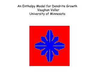
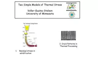
An Enthalpy Model for Dendrite Growth Vaughan Voller University of Minnesota
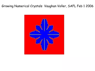
Germs snow-flakes-ice crystals Dendrite grains in material systems Voorhees, Northwestern science.nasa.gov (IACS), EPFL Growing Numerical Crystals Objective: Simulate the growth (solidification) of crystals from a solid seed placed in an under-cooled liquid melt Some Physical Examples
Process REV ~ 1 mm ~5 mm ~0.5 m Computational grid size In terms of the process Sub grid scale
Simulation can be achieved using modest models and computer power Solved in ¼ Domain with A 200x200 grid Box boundaries are insulated Since the thermal boundary layer is thin Boundaries do not affect growth until seed approaches edges Growth of solid seed in a liquid melt Initial dimensionless undercooling T = -0.8 Resulting crystal has an 8 fold symmetry
By changing conditions can generate any number of realistic shapes in modest times PC CPU ~5mins Complete garbage BUT—WHY do we get these shapes ?—WHAT is Physical Bases for Model ? Solution is with a FIXED grid -HOW does the Numerical solution work ? IS the solution “correct” ?
First recognize that there are two under-coolings The bulk liquid is under-cooled, i.e., in a liquid state below the equilibrium liquidus temperature TM The temperature of the solid-liquid interface is undercooled Kinetic vn normal interface velocity Conc. of Solute, m < 0 slope of liquidus • Gibbs Thomson • curvature, g surface tension
On interface n vn Capillary length ~10-9 for metal Angle between normal and x-axis Can describe process with the Sharp Interface Model—for pure material With dimensionless numbers Assumed constant properties Insulated domain Initiated with small solid seed The heat flows from warm solid into the undercooeld liquid drives solidification Preferred growth direction and interplay between curvature and liquid temperature gradient determine Growth rate and shape.
A Diffusive interface model: Usually implies Phase Field—Here we mean ENTHALPY n undercooling The Enthalpy -sum of sensible and latent heats-change continuously and smoothly throughout domain—Hence can write Single Field Eq. For Heat transport (see Tacke 1988, Dutta 2006) Use smooth interpolation for Liquid fraction f across interface Smear out interface f=1 f=0 Can be solved on a Fixed grid
A microstructure model Growth of Equiaxed Crystal In under-cooled melt Sub-grid models Account for Crystal anisotropy and “smoothing” of interface jumps Phase change temperature depends on interface curvature, speed and concentration
Four fold symmetry If f= 0 or f = 1 If 0 < f < 1 curvature Capillary length 10-9 m in Al alloys Local direction Very Simple—Calculations can be done on regular PC Numerical Solution Sub grid constitutive ENTHALPY
At end of time step if solidification Completes in cell i Force solidification in ALL fully liquid neighboring cells. Some Results Physical domain ~ 2-10 microns Typical grid Size 200x200 ¼ geometry seed Initially insulated cavity contains liquid metal with bulk undercooling T0 < 0. Solidification induced by placing solid seed at center.
Tricks and Devices Problem: range of cells with 0 < f < 1 restricted to width of one cell Accuracy in curvature calc? Remedial scheme: smear out f value, e.g., Remedial Scheme: Use nine volume stencil to calculate derivatives
Dendrite shape with 3 grid sizes shows reasonable independence 3.25do (black) 4do (blue) 2.5do (red) e = 0.05, T0 = -0.65 Dimensionless time t = 6000 a = 0.25, b = 0.75
Long term tip dynamics approaches theory Solvabillity (kim et al) BUT results begin to deteriorate if grid is made smaller !!
Verify solution coupling by Comparing with one-d solidification of an under-cooled melt T0 = -.5 Compare with Analytical Similarity Solution Carslaw and Jaeger Front Movement Temperature at dimensionless time t =250
Level Set Kim, Goldenfeld and Dantzig k = 0 (pure), e = 0.05, T0 = -0.55, Dx = d0 Dimensionless time t = 37,600 Looks Right!! Verification 1 Enthalpy Calculation k = 0 (pure), e = 0.05, T0 = -0.65, Dx = 3.333d0 Dimensionless time t = 0 (1000) 6000 Red my calculation for these parameters With grid size
Low Grid Anisotropy The Solid color is solved with a 45 deg twist on the anisotropy and then twisted back —the white line is with the normal anisotropy e = 0.05, T0 = -0.65 Dimensionless time t = 6000 Note: Different “smear” parameters are usedin 00 and 450 case Tip position with time Not perfect: In 450 case the tip velocity at time 6000 (slope of line) is below the theoretical limit.
Sharp Interface Model Use smoothly interpolated Variables across the interface For binary system need to consider – solute transport, discontinuous diffusivities and solutes m Single Domain Eq.
Comparison with one-d Analytical Solution Constant Ti, Ci k = 0.1, Mc = 0.1, T0 = -.5, Le = 1.0 Concentration and Temperature at dimensionless time t =100 Front Movement
Effect of Lewis Number: small Le interface concentration close to C0 k = 0.15, Mc = 0.1, T0 = -.65 • = 0.05, • Dx =3.333d0 All predictions at time t =6000
Concentration k = 0.15, Mc = 0.1, T0 = -.55, Le = 20.0 e = 0.02, Dx = 2.5d0 Profile along dashed line Concentration field at time t = 30,000
FAST-CPU This On This In 60 seconds ! time t = 6000 e = 0.05, T0 = -0.65 a = 0.25, b = 0.75, Dx =4d0
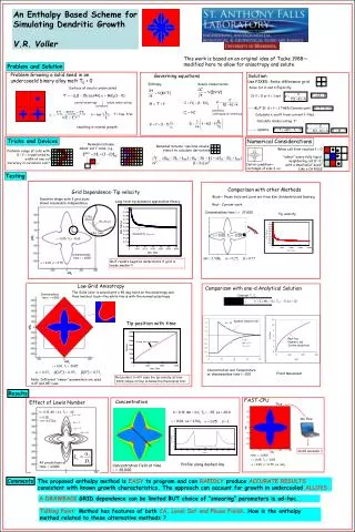
Conclusion –Score card for Dendritic Growth Enthalpy Method (extension of original work by Tacke)
Playing Around A Problem with Noise Multiple Grains-multiple orientations Grains in A Flow Field Thses calculations were performed by Andrew Kao, University of Greenwich, London Under supervision of Prof Koulis Pericleous and Dr. Georgi Djambazov.
Couple with porosity formation ? e.g., shoreline in sedimentary basin 100 km 1000’s of years Extensions: Grain Growth 100 mm seconds Can this work be related to other physical cases ?
NCED’s purpose: to catalyze development of an integrated, predictive science of the processes shaping the surface of the Earth, in order to transform management of ecosystems, resources, and land use The surface is the environment!
Who we are: 19 Principal Investigators at 9 institutions across the U.S. Lead institution: University of Minnesota Research fields • Geomorphology • Hydrology • Sedimentary geology • Ecology • Civil engineering • Environmental economics • Biogeochemistry
Moving Boundaries in Sediment Transport Two Sedimentary Moving Boundary Problems of Interest Shoreline Fans Toes
Examples of Sediment Fans Moving Boundary Badwater Deathvalley 1km How does sediment- basement interface evolve
land surface shoreline ocean x = u(t) x = s(t) a sediment h(x,t) bed-rock b x A Sedimentary Ocean Basin
Melting vs. Shoreline movement An Ocean Basin
Base level 1-D finite difference deforming grid vs. experiment (n calculated from 1st principles) Measured and Numerical results +Shoreline balance
~10km ~10mm Grain Growth in Metal Solidification From W.J. Boettinger “growth” of sediment delta into ocean Ganges-Brahmaputra Delta Is there a connection