Download

1 / 40
400 likes | 489 Vues
Slides Show Summary AGEC 432 Spring 2007. Basic Structure of the Balance Sheet. Assets : Liabilities and Net Worth: Current assets Current liabilities plus Intermediate assets plus Intermediate liabilities

E N D
Basic Structure of the Balance Sheet Assets: Liabilities and Net Worth: Current assets Current liabilities plus Intermediate assets plus Intermediate liabilities plusLong term assets plus long term liabilities plus Net worth (residual value) equals Total assets equals Total liabilities and net worth
Basic Structure of Income Statement Value of farm production Minus Farm expenses Equals Income from operations PlusGain (loss) on sale of intermediate and long term assets Equals Net farm income Plus Non-farm income EqualsIncome (loss) before taxes and extraordinary items Minus Provision for income taxes Equals Income before extraordinary items Plus Extraordinary items Equals Net income
Basic Structure of Cash Flow Statement Cash available MinusCash required Equals Cash available less cash required Plus Savings withdrawals EqualsCash position PlusNet borrowing MinusOther uses of cash Minus Additions to savings Equals Ending cash balance
Monthly Cash Position JanuaryFebruaryMarch Cash available Less Cash required Plus Savings withdrawal Equals Cash position ? ? ? A monthly cash flow statement indicates months of cash flow and surpluses or deficits before borrowing on a LOC… The value of the LOC to request is at least equal to the highest monthly cash flow deficit.
Debt Repayment Capacity Report Farm sources of term debt repayment capacity: Net income $0 $0 Adjustments to net income: Plus Depreciation $0 Less Gain (loss) on sale of assets $0 Less Non-farm income $0 Less Family living withdrawals $0 Less Gifts to others $0 Subtotal $0 $0 Term debt repayment capacity from operations $0 Repayment Capacity from Operations + Repayment margin = repayment capacity – scheduled payments Coverage ratio > 1.0 if repayment margin is positive
Interrelationships Between Financial Statements 2006 Cash Flow Statement Sources of cash: Beginning cash balance Cash receipts from product sales Other sources of cash Total sources of cash Uses of cash: Cash operating expenses Interest payments Principal payments Capital expenditures Withdrawals of cash Other selected uses of cash Ending cash balance Total uses of cash Basic structure: Total sources = total uses 2006 Income Statement Cash receipts from product sales Other income Total income Cash operating expenses Interest payments Other cash expenses Depreciation Total expenses Net income from operations Allowance for taxes Net income Basic structure: EBIT = total income – total expenses + interest payments Balance Sheet 12/31/06 Ending cash balance Other current assets Total current assets Machinery and equipment Buildings and improvements Land Total assets Accounts payable Current loan payment Allowance for taxes Other current liabilities Total current liabilities Remaining balance on loans Total liabilities Equity Basic Structure: Equity = total assets – total Liabilities Equity = Retained net Income + asset revaluations Other statements and schedules: Statement of Change in Owner Equity Depreciable asset schedules
In Class Problem See Problem #1 under Quizzes and Exams link on Website
Slides from Show #3 None… Demonstrated impacts of price and yield shocks to financial statements and financial indicators.
Indicators of growth/survival: Increasing liquidity Increasing solvency Increasing debt repayment capacity Increasing profitability Indicators of potential failure: Declining liquidity Declining solvency Decreasing debt repayment capacity Decreasing profitability Lessons from Beaver Study
Trends in Indicators Failed Failed Failed Failed Source: W. H. Beaver, “Financial Ratios and Predictors of Failure”, Journal of Accounting Research
Historical Analysis • A look backwards like the Beaver study. • Comparison of current performance with past performance. • Recommend doing this at the enterprise level as well as for the farm as a whole. • Reasons underlying unwanted trends such as the declines in last two years?
Comparative Analysis • Comparing current performance with similar operations like the Beaver study. • Benchmark analysis at enterprise level when possible. Similar firms Your firm
Comparative Analysis • Comparing current performance with similar operations like the Beaver study. • Benchmark analysis at enterprise level when possible. • Address reasons why your firm is performing more poorly than other comparable operations before it is too late.
Comparative Analysis • Comparing current performance with similar operations like the Beaver study. • Benchmark analysis at enterprise level when possible. • Address reasons why your firm is performing more poorly than other comparable operations before it is too late.
Comparative Analysis • Comparing current performance with similar operations like the Beaver study. • Benchmark analysis at enterprise level when possible. • Address reasons why your firm is performing more poorly than other comparable operations before it is too late.
Comparative Analysis • Comparing current performance with similar operations like the Beaver study. • Benchmark analysis at enterprise level when possible. • Address reasons why your firm is performing more poorly than other comparable operations before it is too late.
Comparative Analysis • Comparing current performance with similar operations like the Beaver study. • Benchmark analysis at enterprise level when possible. • Address reasons why your firm is performing more poorly than other comparable operations before it is too late.
AB Overhead Rate AB Overhead rate = Overhead per activity ÷ Cost driver per activity Initial status: Activity Cost Pool Overhead Driver AB overhead activity rate Setting up machines $300,000 1,500 setups $200/setup Machining $500,000 50,000 hours $10/hour Inspecting $100,000 2,000 inspection $50/inspection Total $900,000 Step 1: Assigning overhead driver activity to products: Activity Cost Pool Cost driver Driver Product 1Product 2 activity Setting up machines # setups 1,500 500 1,000 Machining Hours 50,000 30,000 20,000 Inspecting # inspections 2,000 500 1,500
AB Overhead Rate Step 1: Assigning overhead driver activity to products: Activity Cost Pool Cost driver Driver Product 1Product 2 activity Setting up machines # setups 1,500 500 1,000 Machining Hours 50,000 30,000 20,000 Inspecting # inspections 2,000 500 1,500 Step 2: Partitioning of overhead: OverheadProduct 1 Product 2___ Setting up machines $300,000 (33%) $100,000 (67%) $200,000 Machining $500,000 (60%) $300,000 (40%) $200,000 Inspecting $100,000 (33%) $25,000 (67%) $75,000 33% = 500/1,500 and 67% = 1,000/1,500
AB Overhead Rate Step 2: Partitioning of overhead: OverheadProduct 1Product 2 Setting up machines $300,000 $100,000 $200,000 Machining $500,000 $300,000 $200,000 Inspecting $100,000$25,000$75,000 Total $900,000 $425,000 $475,000 Step 3: Overhead costs per unit: Units produced 25,000 5,000 Overhead cost per unit $17 $95 Traditional overhead cost per unit*$30 $30 * $900,000 divided by 30,000 units Avoids overstating profitability of some enterprises and understating profitability of others
AB Overhead Rate Product 1 Product 2 COP unit costs with ABC costing: Direct materials $40 $30 Direct labor $12 $12 ABC overhead $17$95 Total unit costs $69 $137 COP unit costs with traditional costing: Direct materials $40 $30 Direct labor $12 $12 Traditional overhead *$30$30 Total unit costs $82 $72 * $900,000 divided by 30,000 units Traditional overhead costing suggests that Product 2 is cheaper to produce than Product 1, which is not true!
Sales Budget Production Budget Direct Materials Budget Direct Labor Budget Overhead Budget Selling and Administrative Expense Budget Budgeted Income Statement Budgeted Cash Flow Statement Capital Expenditure and Cash Budgets Budgeted Balance Sheet
Slides from Show #7 None … showed sensitivity of break even prices and yields to changes in unit costs of production
PRESENT PAST FUTURE • Historical analysis • Comparative analysis • Historical price and yield trends • Pro forma analysis • Forming expectations about future prices, costs and productivity • Ad hoc extrapolations • Projections based upon available outlook data • Projections based upon econometric analysis
Ad Hoc Modeling Approaches • Naïve model – using last year’s prices, costs and yields • Simple linear trend extrapolation of historical prices, costs and yields • Using assumptions made by others
Econometric Model Approach • Capturing future supply/demand impacts on prices and unit costs • Linkages to commodity policy • Linkages to domestic economy • Linkages to the global economy
Timeline Required for Capital Budgeting… Assume it is the year 2000 and John Deere wants to project farm machinery and equipment sales over the next six years to determine if plant expansion is necessary. 2000 2001 2002 2003 2004 2005 2006 Capital budgeting models of investment decisions require projections of the annual farm revenue and cost values over the entire 2001 to 2006 time period.
Conclusions • Econometric models are preferred over naïve models and linear time trend models. • Much more accurate. • Provide much more information (e.g., elasticities). • Allow for sensitivity analysis with independent (exogenous) variables when evaluating potential variability about expected trends.
Some Key Terms • Three types of liquidity (HO #1) • Solvency (HO #1) • Debt repayment capacity (HO #1) • Explicit and implicit cost of capital (HO #5) • Optimal capital structure (HO #1,5) • Historical and comparative analysis (HO #1) • Long run planning curve (HO #2) • Financial risk (HO #2,5) • Payback period (HO #3) • Internal rate of return (HO #3)
More Key Terms • Economic life (HO #3) • Terminal value (HO #3) • Pro forma analysis (HO #4) • Structural econometric simulation (HO #4) • Coefficient of variation (HO #5) • Required rate of return (HO #5) • Business risk premium (HO #5) • Financial risk premium (HO #5)
More Key Terms • Leverage (HO #1 and #5) • Portfolio effect (HO #5) • Negatively correlated cash flows (HO #5) • Weighted average cost of capital (HO #5) • Capital budget constraint (HO #5)