Analysis of Deaths by Horse Kick in the Prussian Army (1875-1894)
This example illustrates a Poisson ANCOVA analysis examining the trend in the number of deaths caused by a horse kick across different units of the Prussian army from 1875 to 1894. The analysis determines if there is a change in risk over time and if there are similar trends in different army units.

Analysis of Deaths by Horse Kick in the Prussian Army (1875-1894)
E N D
Presentation Transcript
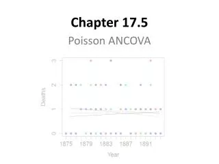
Chapter 17.5 Poisson ANCOVA
Classic Poisson Example • Number of deaths by horse kick, for each of 16 corps in the Prussian army, from 1875 to 1894 • The risk of death did not change over time in Guard Corps. • Is there a similar lack of trend in the 1st,2nd, and 3rd units ?
2. Execute analysis & 3. Evaluate model glm1 <- glm(deaths~year*corps, family = poisson(link=log), data=horsekick)
2. Execute analysis & 3. Evaluate model glm1 <- glm(deaths~year*corps, family = poisson(link=log), data=horsekick)
2. Execute analysis & 3. Evaluate model • glm1 <- glm(deaths~year*corps, family = • poisson(link=log), data=horsekick) • deviance(glm1)/df.residual(glm1) • [1] 1.134671 • Dispersion parameter assumed to be 1 • As a general rule, dispersion parameters approaching 2 (or 0.5) indicate possible violations of this assumption
Side note: Over-dispersion > deviance(glm2)/df.residual(glm2) [1] 4.632645
State population and whether sample is representative. • Decide on mode of inference. Is hypothesis testing appropriate? • State HA / Ho pair, tolerance for Type I error Statistic: Non-PearsonianChisquare(G-statistic) Distribution: Chisquare
7. ANODEV. Calculate change in fit (ΔG) due to explanatory variables. > library(car) > Anova(glm1, type=3) Analysis of Deviance Table (Type III tests) Response: deaths LR ChisqDfPr(>Chisq) year 0.61137 1 0.4343 corps 1.27787 3 0.7344 year:corps 1.27073 3 0.7361
7. ANODEV. Calculate change in fit (ΔG) due to explanatory variables. > Anova(glm1, type=3) … LR ChisqDfPr(>Chisq) year 0.61137 1 0.4343 corps 1.27787 3 0.7344 year:corps 1.27073 3 0.7361 > anova(glm1, test="LR") … Terms added sequentially (first to last) Df Deviance Resid. DfResid. DevPr(>Chi) NULL 79 95.766 year 1 0.00215 78 95.764 0.9630 corps 3 1.14678 75 94.617 0.7658 year:corps 3 1.27073 72 93.347 0.7361
Assess table in view of evaluation of residuals. • Residuals acceptable • Assess table in view of evaluation of residuals. • Reject HA: The four corps show the same lack of trend in deaths by horsekick over two decades (ΔG=1.27, p=0.736) • Analysis of parameters of biological interest. • βyear was not significant – report mean deaths/unit-yr • (56 deaths / 20 years) / 4 units = 0.7 deaths/unit-year
library(pscl) library(Hmisc) library(car) corp.id <- c("G","I","II","III") horsekick <- subset(prussian, corp %in% corp.id) names(horsekick) <- c("deaths","year","corps") glm0 <- glm(deaths ~ 1, family = poisson(link = log), data = horsekick) # intercept only glm1 <- glm(deaths ~ year*corps, family = poisson(link = log), data = horsekick) plot(fitted(glm1),residuals(glm1),pch=16, xlab="Fitted values", ylab="Residuals") plot(residuals(glm1), Lag(residuals(glm1)), xlab="Residuals", ylab="Lagged residuals", pch=16) sum(residuals(glm1, type="pearson")^2)/df.residual(glm1) deviance(glm1)/df.residual(glm1) plot(horsekick$year,horsekick$deaths, pch=16, axes=F, xlab="Year", col=horsekick$corps, ylab="Deaths") axis(1, at=75:94, labels=1875:1894) axis(2, at=0:4) box() Anova(glm1, type=3, test.statistic="LR") anova(glm1, test="LR") species <- read.delim("http://www.bio.ic.ac.uk/research/mjcraw/therbook/data/species.txt") plot(Species~Biomass, data=species, pch=16) lm1 <- lm(Species~Biomass, data=species) plot(fitted(lm1),residuals(lm1), pch=16, xlab="Fitted values", ylab="Residuals", main="GLM") glm2<-glm(Species~Biomass, data=species, family=poisson) plot(fitted(glm2),residuals(glm2), pch=16, xlab="Fitted values", ylab="Residuals", main="GzLM") deviance(glm2)/df.residual(glm2)