PBF Zagreb, Croatia, 25.01. 2012 Structural Equation Modeling - data analyzing -

1. PBF Zagreb, Croatia, 25.01. 2012Structural Equation Modeling- data analyzing - Tatjana Atanasova – Pachemska, „Goce Delcev” University - Shtip, Macedonia

2. Essentials Purpose of this lecture is to provide a very brief presentation of the things one needs to know about SEM before learning how apply SEM.

3. Outline I. Essential Points about SEM II. Structural Equation Models: Form and Function III. Research Examples

4. What is SEM? • Structural equation modeling (SEM) is a series of statistical methods that allow complex relationships between one or more independent variables and one or more dependent variables. • Though there are many ways to describe SEM, it is most commonly thought of as a hybrid between some form of analysis of variance (ANOVA)/regression and some form of factor analysis. In general, it can be remarked that SEM allows one to perform some type of multilevel regression/ANOVA on factors. We should therefore be quite familiar with univariante and multivariate regression/ANOVA as well as the basics of factor analysis to implement SEM for our data.

5. SEM goes beyond factor analysis to test expected relationships between a set of variables and the factors upon which they are expected to load. As such, it is considered to be a confirmatory tool • SEM also goes beyond multiple regression to demonstrate how those independent variables contribute to explanation of the dependent variable. It models the direction of relationshipswithin a multiple regression equation. • The goal of SEM is to identify a model that makes theoretical sense, is a good fit to the data . The model developed should be theory-driven, or based on past research.

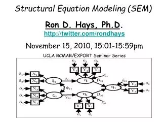
6. 1 11 y1 graphical form x1 equational form y1 = γ11x1 + ζ1 1. SEM is a form of graphical modeling, and therefore, a system in which relationships can be represented in either graphical or equational form. I. SEM Essentials ( SEM language): 2. An equation is said to be structural if there exists sufficient evidence from all available sources to support the interpretation that x1 has a causal effect on y1.

7. Complex Hypothesis x1 y3 ζ3 y1 y2 ζ1 ζ2 • e.g. • y1 = γ11x1 + ζ1 • y2 = β 21y1 + γ 21x1 + ζ 2 • y3 = β 32y2 + γ31x1 + ζ 3 Corresponding Equations 3. Structural equation modeling can be defined as the use of two or more structural equations to represent complex hypotheses.  (gamma) used to represent effect of exogenous on endogenous.  (beta) used to represent effect of endogenous on endogenous

8. Some preliminary terminology will also be useful. The following definitions regarding the types of variables that occur in SEM allow for a more clear explanation of the procedure: • Variables that are not influenced by another other variables in a model are called exogenous (independent) variables. • Variables that are influenced by other variables in a model are called endogenous variables. • A variable that is directly observed and measured is called an indicator (manifest) variable. There is a special name for a structural equation model which examines only manifest variables, called path analysis. • A variable that is not directly measured is a latent variable. The “factors” in a factor analysis are latent variables.

9. Drawing our hypothesized model: procedures and notation The most important part of SEM analysis is the causal model we are required to draw before attempting an analysis. The following basic, general rules are used when drawing a model: • Rule 1. Latent variables/factors are represented with circles and measured/manifest variables are represented with squares.

10. Rule 2. Lines with an arrow in one direction show a hypothesized direct relationship between the two variables. It should originate at the causal variable and point to the variable that is caused. Absence of a line indicates there is no causal relationship between the variables. Rule 3. Lines with an arrow in both directions should be curved and this demonstrates a bi-directional relationship (i.e., a covariance). Rule 3a.Covariance arrows should only be allowed for exogenous variables.

11. Rule 4. For every endogenous variable, a residual term should be added in the model. Generally, a residual term is a circle with the letter E written in it, which stands for error. Rule 4a. For latent variables that are also endogenous, a residual term is not called error in the lingo of SEM. It is called a disturbance, and therefore the “error term” here would be a circle with a D written in it, standing for disturbance.

13. SEM Process A suggested approach to SEM analysis proceeds through the following process: • review the relevant theory and research literature to support model specification • specify a model (e.g., diagram, equations) • determine model identification (e.g., if unique values can be found for parameter estimation; the number of degrees of freedom df, for model testing is positive)

14. select measures for the variables represented in the model • • collect data • • conduct preliminary descriptive statistical analysis (e.g., scaling, missing data, collinearity issues, outlier detection) • • estimate parameters in the model • • assess model fit • • respecify the model if meaningful • • interpret and present results.

15. Examples Figure 1. Regression Model (math achievement at age 10, reading comprehension achievement at age 12, and mother’s educational level predicting math achievement at age 12).

16. Figure 2. Revised model (math achievement at age 10, reading comprehension at age 12 predict math achievement at age 12; indirect effect of mother’s educational level and math achievement at age 10).

17. Figure 3. Structural Equation Model - Relationship between academic and job constructs

18. Contemporary Wright (1918) path analysis Joreskog (1973) SEM factor analysis A Grossly Oversimplified History of SEM Spearman (1904) Lee (2007) testing alt. models r, chi-square likelihood Conven- tional Statistics Pearson (1890s) Fisher (1922) Neyman & E. Pearson (1934) Bayesian Analysis Bayes & LaPlace (1773/1774) Raftery (1993) MCMC (1948-) Note that SEM is a framework and incorporates new statistical techniques as they become available (if appropriate to its purpose)

19. The LISREL Synthesis Karl Jöreskog 1934 - present Key Synthesis paper- 1973

20. The Methodological Side of SEM

21. How do data relate to learning? multivariate descriptive statistics multivariate data modeling realistic predictive models SEM univariate descriptive statistics univariate data modeling Data exploration, methodology and theory development abstract models more detailed theoretical models Understanding of Processes modified from Starfield and Bleloch (1991)

22. SEM is one of the few applications of statistical inference where the results of estimation are frequently “you have the wrong model!”. This feedback comes from the unique feature that in SEM we compare patterns in the data to those implied by the model. This is an extremely important form of learning about systems.

23. AMOS Graphics AMOS (Analysis of MOments Structures) is a statistical package specializing in structural equation modeling. AMOS builds measurement, structural or full structural models. It tests, modifies and retests models. AMOS also tests alternate models, equivalence across groups or samples, as well as hypotheses about means and intercepts. It handles missing data using Maximum Likelihood (ML) estimation and provides bootstrapping procedures. Results obtained in AMOS are comparable to those obtained through other SEM packages.

24. Five Steps to SEM • Model specification; • Model identifiability; • Measure selection, data collection, cleaning and preparation; • Model analysis and evaluation; • Model respecification

25. Model specification involves mathematically or diagrammatically expressing hypothesized relationships among a set of variables. The challenge at this step is to include all endogenous and exogenous variables, (including moderators and mediators), that are expected to contribute to central endogenous variables. Exclusion of important variables may result in the misestimation of endogenous variables. The extent of misestimation increases with the strength of the correlation between missing and endogenous variables. Whilst it is impossible to include all variables that contribute to the prediction of endogenous variables, it is possible to identify the main ones through careful examination of relevant theory and past research A second challenge is to determine the direction of relationships between pairs of variables in the SEM model. Actual direction is debatable, especially where manifest variables are measured at the same point in time

26. Step 2: Model Identifiability Specified models need to be checked for identifiability. A model is theoretically identifiable if there is a unique solution possible for it and each of its parameters. If a model is not identifiable, then it has no unique solution and SEM software will fail to converge. Such models need to be respecified to be identifiable. The maximum number of parameters that can be specified in the model is equivalent to the number of unique variances and covariances that can be found in its underlying covariance matrix. If, for example, there are four variables (say: A, B, C, and D), a covariance matrix has four unique variances (one for each variable) along with six unique covariances (AB, AC, AD, BC, BD and CD), giving a total of ten unique parameters. (See figure).

27. A B C D A Var(A) B Cov(AB) Var(B) C Cov(AC) Cov(BC) Var(C ) D Cov(AD) Cov(BD) Cov(CD) Var(D) A Covariance Matrix With Four Variables, A, B, C and D. Note: For four variables, there are four unique variances and six unique covariances, giving a maximum of ten parameters estimable with SEM.

29. Step 3: Measure Selection, Data Collection, Cleaning and Preparation Step 3 has four substeps: measure selection, data collection, data cleaning and data preparation Step 3a - Measure Selection Manifest variables are estimates of the underlying latent constructs they purport to measure. It is therefore recommended that each latent construct be measured by at least two manifest variables. Measures selected need to demonstrate good psychometric properties. They need to be both “reliable” and “valid” measure.

30. Coefficients of 0.8 or above suggest good reliability, whilst those in the range of 0.7 to 0.8 suggest adequacy. Coefficients below 0.5 should be avoided or improved before use in research. • Validity is assessed by examining its content, criterion-related, convergent or discriminant validities • Content validity exists when experts agree that the measure is tapping into the relevant domain. • Criterion-related validity assesses whether a measure taps into a particular domain, as assessed against some set criteria

31. Step 3b - Data Collection • A sufficiently large sample needs to be drawn in order to analyse the model specified at Step 1. The sample drawn should be ten times the number of model parameters to be estimated, with a minimum of 200 cases. If planning to divide the sample in two for model development and testing purposes, then each half sample needs to be sufficiently large. Moreover, expected response rates should be factored into consideration when drawing the sample.

32. Step 3c - Data “Cleaning” • The acronym GIGO (Garbage In, Garbage Out) highlights the importance of checking the veracity and integrity of data entry. In statistical terms, doing so ensures that data is “clean” before proceeding further. • Checking each datapoint of a large dataset may be tedious. However, it is possible to check (and correct) the first five or ten cases and extrapolating their accuracy rate to the remaining cases in the dataset. If accuracy is less than, say, 95%, the data could be reentered using a double entry method.

33. II. Structural Equation Models: Form and Function A. Anatomy of Observed Variable Models

34. Some Terminology path coefficients direct effect of x1 on y2 21 x1 y2 11 21 2 y1 exogenous variable 1 endogenous variables indirect effect of x1 on y2 is11times 21

35. model B, which has paths between all variables is “saturated” (vs A, which is “unsaturated”) A B x1 y1 y2 x1 y1 y2 ζ2 ζ2 ζ1 ζ1 C D x1 y2 x1 y2 ζ2 ζ2 x2 y1 x2 y1 ζ1 ζ1 nonrecursive

36. First Rule of Path Coefficients: the path coefficients for unanalyzed relationships (curved arrows) between exogenous variables are simply the correlations (standardized form) or covariances (unstandardized form). x1x2y1 ----------------------------- x1 1.0 x2 0.40 1.0 y1 0.50 0.60 1.0 x1 y1 .40 x2

37. Second Rule of Path Coefficients: when variables are connected by a single causal path, the path coefficient is simply the standardized or unstandardized regression coefficient (note that a standardized regression coefficient = a simple correlation.) 11 = .50 21 = .60 x1 y1 y2 ------------------------------------------------- x1 1.0 y1 0.50 1.0 y2 0.30 0.60 1.0 x1 y1 y2

38. Third Rule of Path Coefficients: strength of a compound path is the product of the coefficients along the path. .50 .60 x1 y1 y2 Thus, in this example the effect of x1 on y2 = 0.5 x 0.6 = 0.30 Since the strength of the indirect path from x1 to y2 equals the correlation between x1 and y2, we say x1 and y2 are conditionally independent.

39. What does it mean when two separated variables are not conditionally independent? x1y1y2 ------------------------------------------------- x1 1.0 y1 0.55 1.0 y2 0.50 0.60 1.0 r = .55 r = .60 x1 y1 y2 0.55 x 0.60 = 0.33, which is not equal to 0.50

40. The inequality implies that the true model is additional process x1 y2 y1 Fourth Rule of Path Coefficients: when variables are connected by more than one causal pathway, the path coefficients are "partial" regression coefficients. Which pairs of variables are connected by two causal paths? answer: x1 and y2 (obvious one), but also y1 and y2, which are connected by the joint influence of x1 on both of them.

41. And for another case: x1 y1 x2 A case of shared causal influence: the unanalyzed relation between x1 and x2 represents the effects of an unspecified joint causal process. Therefore, x1 and y1 connected by two causal paths x2 and y1 likewise.

42. How to Interpret Partial Path Coefficients: The Concept of Statistical Control .31 x1 y2 The effect of y1 on y2 is controlled for the joint effects of x1. .48 .40 y1 Grace, J.B. and K.A. Bollen 2005. Interpreting the results from multiple regression and structural equation models. Bull. Ecological Soc. Amer. 86:283-295.

43. Fifth Rule of Path Coefficients: paths from error variables are correlations or covariances. R2 = 0.44 .31 x1 y2 .73 R2 = 0.16 .40 .48 2 y1 .56 equation for path from error variable .92 1 .84 alternative is to show values for zetas, which = 1-R2

44. Now, imagine y1 and y2 are joint responses R2 = 0.25 y2 2 .50 x1y1y2 ------------------------------- x1 1.0 y1 0.40 1.0 y2 0.50 0.60 1.0 x1 .40 y1 1 R2 = 0.16 Sixth Rule of Path Coefficients: unanalyzed residual correlations between endogenous variables are partial correlations or covariances.

45. .40 R2 = 0.25 y2 2 .50 x1 .40 y1 1 the partial correlation between y1 and y2 is typically represented as a correlated error term R2 = 0.16 This implies that some other factor is influencing y1 and y2

46. Seventh Rule of Path Coefficients:total effect one variable has on another equals the sum of its direct and indirect effects. x1 y2 ζ2 x2 y1 Total Effects: .15 x1x2 y1 ------------------------------- y1 0.64 -0.11 --- y2 0.32 -0.03 0.27 ζ1 Eighth Rule of Path Coefficients: sum of all pathways between two variables (causal and noncausal) equals the correlation/covariance. note: correlation between x1 and y1 = 0.55, which equals 0.64 - 0.80*0.11 .64 .80 .27 -.11

47. Suppression Effect - when presence of another variable causes path coefficient to strongly differ from bivariate correlation. x1 x2 y1 y2 ----------------------------------------------- x11.0 x20.80 1.0 y1 0.55 0.40 1.0 y2 0.30 0.23 0.35 1.0 x1 y2 ζ2 x2 y1 .15 ζ1 .64 .80 .27 -.11 path coefficient for x2 to y1 very different from correlation, (results from overwhelming influence from x1.)

48. II. Structural Equation Models: Form and Function B. Anatomy of Latent Variable Models

49. Latent Variables Latent variables are those whose presence we suspect or theorize, but for which we have no direct measures. fixed loading* Intelligence 1.0 1.0 ζ IQ score latent variable observed indicator error variable *note that we must specify some parameter, either error, loading, or variance of latent variable.

50. Latent Variables (cont.) Purposes Served by Latent Variables: (1) Specification of difference between observed data and processes of interest. (2) Allow us to estimate and correct for measurement error. (3) Represent certain kinds of hypotheses.