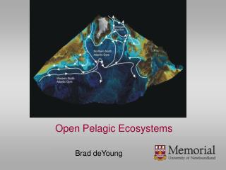
Brad deYoung
Open Pelagic Ecosystems. Brad deYoung. Roadmap. Ecosystem structure – considerations of the issues and how to think about them Regime shifts in the ocean – examples of some observed behaviour that we do not quite understand Variability and modelling of marine ecosystems, some examples.

Brad deYoung
E N D
Presentation Transcript
Open Pelagic Ecosystems Brad deYoung
Roadmap • Ecosystem structure – considerations of the issues and how to think about them • Regime shifts in the ocean – examples of some observed behaviour that we do not quite understand • Variability and modelling of marine ecosystems, some examples
Top down view more life history driven >> structured models Challenge : With a target species focus to couple structured models (even if not IBM) and predators and prey below which may have different model structures or data Bottom up view more process driven – represent metabolism, mass-balance Simplified life history model or data Structured population model All models are wrong, but some models are useful.George Box Mass balance models –NPpZzD … Nutrient Pool
What criteria do we use to simplify our ecosystem food web? Selection of target speciesA mixture of theory, observation and pragmatism • Functionally important/ecologically significant • Extensive data sets (spatial and temporal) • Choose a food web in which the first PCA contains relatively few species • Concurrence with other relevant data sets • Understanding of life history • Widely distributed/across the basin • Economic and societal importance • Well resolved taxonomy • …
Modelling can be driven by • data exploration (see right) • process exploration • forecast simulations Low frequency changes are more important than we once thought The long-period changes lead to larger spatial scales >> basins Shifts in physical (temperature, mixed layer depth, …) and biological properties (phytoplankton, zooplankton,…) Chavez et al. Science (2002)
Predation Key taxa Feeding Number of state variables Detail of resolution Trophic complexity –maintaining fidelity to life history as it becomes more complex and also more difficult to model Top predators Trophic level Bacteria Probable number of species ICES - Report of the Study Group on spatial and temporal integration, University of Strathclyde, Glasgow, Scotland, 14-18 June 1993. ICES CM 1993/L:9, (1993).
Physical Ocean Zooplankton/fisheries focus Predators Life History Trophic level Without Life History Phytoplankton/nutrient focus Chemistry Functional Complexity deYoung et al. Science. 2004
Top-down predation Challenge lies in coupling the structured and unstructured models and data Coupling with the structured components will likely be one-way Zooplankton Focus Open Ocean Shelf Planktivorous Predators Fish - sandlance, capelin, herring, sprat, mackerel, Norway put, blue whiting; Zooplankton - gelatinous, euphausiids Fish - myctophids, redfish, herring, blue whiting; Zooplankton - gelatinous, euphausiids Zooplankton – Structured population representations of key basin distributed species – variously, particularly congeneric Calanus spp., euphausiids Unstructured competitors for structured zooplankton Food for zooplankton: Microzooplankton, diatoms, non-diatoms, Phaeocystis Physics and chemistry – high resolution large scale circulation, coupling between global, basin and shelf models First Order Horizontal Structure
Low frequency ‘cycles’ are not likely as linear as they may appear • linear shifts, i.e. nothing special happening • abrupt shifts but reversible in principle • non-linear shifts that are not easily reversible • how linear is the fundamental behaviour that we are trying to represent? Anderson et al. TREE 2008 deYoung et al. Prog. Ocgy. ( 2004), TREE 2008
DEFINITION OF THE REGIME SHIFT Working definition : a regime shift is a relatively abrupt change between contrasting persistent states in an ecosystem
Erosion of resilience Environmental state Erosion of resilience Environmental driver
Review of a few examples of regime shifts in pelagic ecosystems • Scotian Shelf – driven primarily by fishing, cascading trophic impacts • North Sea – combined drivers: natural=biogeographic shift and human=fishing • North Pacific – complex natural state change(s) Explore characteristics of the drivers and response of differing examples – time and space scales, trophic structure, predictability
-30% +30% Scotian Shelf – Frank et al. 2005
Colour display of 60+ indices for Eastern Scotian Shelf Grey seals, pelagic fish abundance, invertebrate landings, fish species richness, phytoplankton Grey seals - adults Pelagic fish - #’s Pelagic:demersal #’s Pelagic:demersal wt. Inverts - $$Pelagics - wtDiatoms Grey seals – pups Pelagics - $$ Greenness Dinoflagellates Fish diversity – richness 3D Seisimic (km2) Gulf Stream position Stratification anomaly Diatom:dinoflagellate Sea level anomaly Volume of CIL source water Inverts – landings Bottom water < 3 C Sable winds (Tau) SST anomaly (satellites) chlorophyll – CPR Temperature of mixed layer NAO Bottom T – Emerald basin Copepods – Para/Pseudocal Shelf-slope front position Storms Bottom T – Misaine bank Groundfish landings Haddock – length at age 6 Bottom area trawled (>150 GRT) Cod – length at age 6 Average weight of fish Community similarity index PCB’s in seal blubber Relative F Pollock – length at age 6 Calanus finmarchicus Groundfish biomass – RV Pelagics – landings Silver hake – length at age Condition – KF Depth of mixed layer Condition – JC Proportion of area – condition RIVSUM Sigma-t in mixed layer Oxygen Wind stress (total) Wind stress (x-direction) Wind stress amplitude SST at Halifax Groundfish - $$ Salinity in mixed layer Ice coverage Wind stress (Tau) Number of oil&gas wells drilled Nitrate Groundfish fish - #’s Shannon diversity index –fish Seismic 2D (km) Red – below average Green – above average Bottom temp., exploitation, groundfish biomass & landings, growth-CHP, avg. fish weight, copepods 1970 1975 1980 1985 1990 1995 2000
Scotian Shelf – top down story Top Predators (Piscivores) + Forage (fish+inverts) (Plankti-,Detriti-vores) - Zooplankton (Herbivores) + Phytoplankton (Nutrivores) - Frank et al. 2004/2005 Science et al.
Physical forcing – air temperature - but there are dozens, and dozens of other such time series
The technique of Hare and Mantua has been criticized as being subject to false positives – taking the normalized variance anomalies of many different time series with red spectra can lead to ‘apparent’ shifts The lack of sufficient clear data is one problem The time series are too short The regimes are likely never completely in equilibrium Many different possible states are likely Anderson et al. Reviewed the different approaches, and confirm the basic result of Hare and Mantua
North Sea regime shift – a mixture of biogeography, environmental change and fishing Line in black: warm-temperate species Line in red: temperate species 12 5 11 4.5 M O N T H S 10 4 9 8 3.5 7 3 6 2.5 5 2 4 1.5 3 2 1 1 58 62 66 70 74 78 82 86 90 94 98 Years Mean number of calanoid species per CPR sample Before 1980 After 1980
Gadoid species (cod) Flatfish plankton change plankton change salinity SST NHT anomalies Westerly wind
Beaugrand & Ibanez (in press, MEPS) Beaugrand G (2004) Progress in Oceanography
Beaugrand & Ibanez (in press, MEPS) Beaugrand G (2004) Progress in Oceanography
Long-term changes in the abundance of two key species in the North Sea Percentage of C. helgolandicus Reid et al. (2003)
Consequences of plankton changes on higher trophic level Abundance of C. finmarchicus Abundance of C. helgolandicus Mismatch between the timing of calanus prey and larval cod Beaugrand, et al. (2003) Nature. Vol. 426. 661-664.
But there is also a significant influence of fishing – how much??
North Sea - dynamics Ocean circulation Biogeographic shift Meteorological/oceanographic forcing Fishing Ecosystem status and function Ocean conditions
Seasonal sea surface temperature anomalies over the North Atlantic for 2006 From the NOAA Optimum Interpolation SSTv2 dataset, provided by the NOAA-CIRES Climate Diagnostics Center, USA. The anomaly is calculated with respect to normal conditions for the period 1971–2000. The data are produced on a one-degree grid from a combination of satellite and in situ temperature data. Regions with ice over for >50% of the averaging period are left blank. ICES Report on Ocean Climate 2006. Prepared by the Working Group on Oceanic Hydrography Sarah L. Hughes and N. Penny Holliday, Editors. ICES cooperative research report no. 289 special issue September 2007 (from Figure 4).
Biological consequences expected under climatic warming Or changes in water mass structure. • Changes in the range and spatial distribution of species. • Shifts in the location of biogeographical boundaries, provinces, • and biomes. • Change in the phenology of species (e.g. earlier reproductive season). • Modification in dominance (e.g. a key species can be replaced by • another one). • Change in diversity. • Change in other key functional attributes for marine ecosystems. • Change in structure and dynamics of ecosystem with possible • regime shifts. Expected Result: Major impact for marine exploited resources and biogeo- chemical processes (e.g. sequestration of CO2 by the ocean).
Long-term changes in the mean number of species per assemblage based on three periods: 1958-1981, 1982-1999, and 2000-2002. Warm-water species have extended their distribution northwards by more than 10° of latitude, while cold-water species have decreased in number and extension. (Beaugrand, G. ICES Journal of Marine Science, 62: 333-338 (2005)
Calanus finmarchicus in the North Atlantic - open ocean, deep and shallow, spreads out onto shelf, for some species some evidence for genetic separation, copepods key organisms for food web, coupled with circulation
Diapause depth – how deep do they go? Heath et al. (2004)
Calanus in the Labrador Sea Biological model – with a lot of detail on copepod development and growth – in this case the numerical organism eats satellite (SeaWifs) chlorphyll data The physical model represents the seasonal circulation in the Labrador Sea and the organisms are carried around in it In the vertical the zooplankton behaviour determines their position Non-diapausing individuals • Population achieves maximum growth rate when emergence is 1 month prior to the spring bloom • Timing of population peaks is closely matched observations Diapausing individuals Phytoplankton Temperature Tittensor et al. Fish. Ocgy. 2004
May January July November Advection • Latitudinally dependent emergence, starting in South (March) and later to the North (May) • only start out in water > 1000m deep (none on the shelf) • results in a peak in the centre of the Labrador Sea • some Calanus move up onto the shelf • Locally sustainable population Tittensor et al. Fish. Ocgy. 2004
Model design for the North Atlantic Calanus problem – Heath, Speirs, Gurney et al. (2005)
Entry Exit H1 Low food Development at depth H2 Low food Photoperiod Use the model to test different hypotheses of diapause – a process for which we have no direct process model
OWS Mike - hypothesis test Surface Copepodites Diapausers H1 H1 H3 H3 Newly surfaced overwinterers Sharp drop at awakening No diapausers in spring
Long-term spatial structure and advection through the basin • Preliminary conclusion is hat biology dominates over circulation • Requires some ‘adjusting’ different parts of the basin • Is able to reproduce the population dynamics at the basin scale – for the first time. Year 1 Year 3 Year 6 Speirs et al. Fish. Ocgy. (2005)
If god had consulted me before embarking on the creation, I would have suggested something simpler. Alfonso of Castile (15th century)