Download

1 / 46
460 likes | 668 Vues
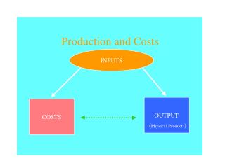
Chapter 1: Inputs and Production Functions. Definitions. Definition: Productive resources, such as labor and capital equipment, that firms use to manufacture goods and services are called Definition: The amount of goods and services produces by the firm is the firm’s

E N D
Definitions Definition: Productive resources, such as labor and capital equipment, that firms use to manufacture goods and services are called Definition: The amount of goods and services produces by the firm is the firm’s Definition: transforms a set of inputs into a set of outputs Definition: determines the quantity of output that is feasible to attain for a given set of inputs. inputs or factors of production. output. Production Technology
Definitions Continued Definition: tells us the maximum possible output that can be attained by the firm for any given quantity of inputs. The production function • Example: Q = f(L,K,M) • Example: Q = f(P,F,L,A) • Example: Chips = f1(L,K,M) • = f2(L,K,M)
Notes on the Production Function • Definition: is attaining the maximum possible output from its inputs (using whatever technology is appropriate) A technically efficient firm
Q Example: The Production Function and Technical Efficiency Production Function Q = f(L) D • C • • B Production Set • A L
production set. • Definition: The feasible but inefficient points below the production function make up the firm’s • Are firms technically efficient? • Shirking, “perquisites” • Strategic reasons for technical inefficiency • Imperfect information on “best practices” • “63% efficient”
The variables in the production function are flows (the amount of the input used per unit of time), not stocks (the absolute quantity of the input). • Example: stock of capital is the total factory installation; flow of capital is the machine hours used per unit of time in production (including depreciation). • Capital refers to physical capital • (definition: goods that are themselves produced goods) and not financial capital (definition: the money required to start or maintain production).
Example: Q = (1/192)[K2-(1/36)K3][L2 – (1/36)L3] Q = K1/2L1/2
Definition: of an input is the change in output that results from a small change in an input holding the levels of all other inputs constant. The marginal product MPL = Q/L (holding constant all other inputs) MPK = Q/K (holding constant all other inputs) Example: MPL = (1/2)L-1/2K1/2 MPK = (1/2)K-1/2L1/2
Definition: The average product of an input is equal to the total output that is to be produced divided by the quantity of the input that is used in its production: APL = Q/L APK = Q/K Example: APL = [K1/2L1/2]/L = K1/2L-1/2 APK = [K1/2L1/2]/K = L1/2K-1/2 Definition: The law of diminishing marginal returns states that marginal products (eventually) decline as the quantity used of a single input increases.
Links between Total, Average and Marginal Magnitudes Student Height (CM) Arrival Height Total Average Marginal 1 160 160 160 160 2 180 340 170 180 3 190 530 176.67 190 4 150 680 170 150 5 150 830 166 150 "TP" "AP" "MP"
When a total magnitude is rising, the corresponding marginal magnitude is positive. • When an average magnitude is falling, the corresponding marginal magnitude must be smaller than the average magnitude.
Q Example: Total, Average and Marginal Magnitudes L MPL maximized TPL maximized where MPL is zero. TPL falls where MPL is negative; TPL rises where MPL is positive. APL MPL APL maximized L
Isoquants Definition: An isoquant traces out all the combinations of inputs (labor and capital) that allow that firm to produce the same quantity of output.
K Example: Isoquants Q = 10 Slope=K/L L 0
K Example: Isoquants All combinations of (L,K) along the isoquant produce 20 units of output. Q = 20 Q = 10 Slope=K/L L 0
Definition: The marginal rate of technical substitution measures the amount of an input, L, the firm would require in exchange for using a little less of another input, K, in order to just be able to produce the same output as before. MRTSL,K = -K/L (for a constant level of output) Marginal products and the MRTS are related: MPL(L) + MPK(K) = 0 => MPL/MPK = -K/L = MRTSL,K therefore,
If both marginal products are positive, the slope of the isoquant is negative... • If we have diminishing marginal returns, we also have a diminishing marginal rate of technical substitution. For many production functions, marginal products eventually become negative. Why don't most graphs of isoquants include the upwards-sloping portion?
K Example: The Economic and the Uneconomic Regions of Production Isoquants MPK < 0 Q = 20 MPL < 0 Q = 10 L 0
Definition: The elasticity of substitution, , measures how the capital-labor ratio, K/L, changes relative to the change in the MRTSL,K. = [(K/L)/MRTSL,K]x[MRTSL,K/(K/L)] • Example:Suppose that… • MRTSAL,K = 4, KA/LA = 4 • MRTSBL,K = 1, KB/LB = 1 • MRTSL,K = MRTSBL,K - MRTSAL,K = -3 • = [(K/L)/MRTSL,K]x[MRTSL,K/(K/L)] • = (-3/-3)(4/4) = 1
Example: The Elasticity of Substitution K "The shape of the isoquant indicates the degree of substitutability of the inputs…" = 0 = 1 = 5 = L 0
Technological Progress Definition:Technological progress (or invention) shifts the production function by allowing the firm to achieve more output from a given combination of inputs (or the same output with fewer inputs). Neutral technological progress shifts the isoquant corresponding to a given level of output inwards, but leaves the MRTSL,K unchanged along any ray from the origin
Technological Progress Ctd... Labor saving technological progress results in a fall in the MRTSL,K along any ray from the origin Capital saving technological progress results in a rise in the MRTSL,K along any ray from the origin.
Example: “neutral technological progress” K Q = 100 ante Q = 100 post MRTS remains same K/L L
Example: Labor Saving Technological Progress K Q = 100 ante Q = 100 post MRTS gets smaller K/L L
Example: “capital saving technological progress” K Q = 100 ante Q = 100 post MRTS gets larger K/L L
Example: Initially a firm’s production function takes the form: • Q = 500[L+3K] • its production function becomes: • Q = 1000[.5L + 10K] • MPL1= 500 MPL2 = 500 • MPK1= 1500 MPK2 = 10,000 • So MRTSL,K has decreased (“labor saving technological progress has occurred”)
Example: Chemicals in the UK Evidence of materials-saving and capital using technological progress… In other words, evidence that MPM DECREASED relative to the MP0 …and… MPK INCREASED relative to MP0. Further, 30% growth of input productivity attributable to technological progress
Returns To Scale • How much will output increase when ALL inputs increase by a particular amount? • RTS = [%Q]/[%(all inputs)] If a 1% increase in all inputs results in a greater than 1% increase in output, then the production function exhibits increasing returns to scale. If a 1% increase in all inputs results in exactly a 1% increase in output, then the production function exhibits constant returns to scale. If a 1% increase in all inputs results in a less than 1% increase in output, then the production function exhibits decreasing returns to scale.
K Example: Returns to Scale 2K Q = Q1 K Q = Q0 L 0 L 2L
Notes: • The marginal product of a single factor may diminish while the returns to scale do not • Returns to scale need not be the same at different levels of production • Many production processes obey the cube-square rule, resulting in increasing returns to scale.
Example: Q1 = AL1K1 • Q2 = A(L1)(K1) • = + AL1K1 • = +Q1 • so returns to scale will depend on the value of +. • + = 1 … CRS • + <1 … DRS • + >1 … IRS • What are the returns to scale of: • Q1 = 500L1+400K1?
Example: Electric Power Generation 1950s, estimate Q = ALKF …find ++>1 more recently, find this sum equals 1 • Example: Returns to scale in oil pipelines • Q = AH.37D1.73 • Increasing returns to scale in horsepower and diameter
Special Production Functions • 1. Linear Production Function: • Q = aL + bK • MRTS constant • Constant returns to scale • =
K Example: Linear Production Function Q = Q1 Q = Q0 L 0
O Example: Fixed Proportion Production Function 2 Q = 2 (molecules) Q = 1 (molecule) 1 0 H 2 4
3. Cobb-Douglas Production Function: Q = aLK • if + > 1 then IRTS • if + = 1 then CRTS • if + < 1 then DRTS • smooth isoquants • MRTS varies along isoquants • = 1
K Example: Cobb-Douglas Production Function Q = Q1 Q = Q0 0 L
4. Constant Elasticity of Substitution Production • Function: Q = [aL+bK]1/ • Where = (-1)/ • if = 0, we get Leontief case • if = , we get linear case • if = 1, we get the Cobb-Douglas case
Summary • 1. Production function is analogous to utility function and is analyzed by many of the same tools. 2. One of the main differences is that the production function is much easier to infer/measure than the utility function. Both engineering and econometric techniques can be used to do so. • 3.Technological progress shifts the production function by allowing the firm to achieve more output from a given combination of inputs (or the same output with fewer inputs).
Summary Continued • 4. Returns to Scale is a long run concept: It refers to the percentage change in output when all inputs are increased a given percentage. 5. The production function is cardinal, not ordinal