Efficient Pricing with Increasing Returns to Scale and Externality
980 likes | 1.01k Vues
Analyzing public policy through utility theory for subsidies and pollution control. Optimal pricing for activities with increasing returns to scale and externalities is explored.

Efficient Pricing with Increasing Returns to Scale and Externality
E N D
Presentation Transcript
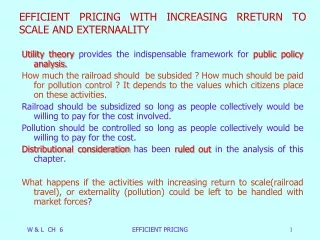
EFFICIENT PRICING WITH INCREASING RRETURN TO SCALE AND EXTERNAALITY Utility theory provides the indispensable framework for public policy analysis. How much the railroad should be subsided ? How much should be paid for pollution control ? It depends to the values which citizens place on these activities. Railroad should be subsidized so long as people collectively would be willing to pay for the cost involved. Pollution should be controlled so long as people collectively would be willing to pay for the cost. Distributional consideration has been ruled out in the analysis of this chapter. What happens if the activities with increasing return to scale(railroad travel), or externality (pollution) could be left to be handled with market forces? EFFICIENT PRICING
EFFICIENT PRICING WITH INCREASING RRETURN TO SCALE AND EXTERNAALI Because of falling marginal and average cost the increasing return to scale activities would be prone to(natural) monopolies, if it were left to be handled by the free market. Because of the difference between private and social cost, pollution will not be optimally controlled(there would be too much pollution), if it will be left to be handled by the free market. Because , one man’s actions affect others without his being forced by the price mechanism to take the effects into account. In the case of externality the efficient amount of output will be found from Σ MRS = MRT, which can not be achieved by the free market operation In this chapter we examine the meaning of efficient pricing in different activities, and different situation(externality and increasing return to scale). EFFICIENT PRICING
First – Best Pricing and investment. Typical increasing return to scale activity ; building the bridge. The bridge cost f units of y to build and is able to provide up to g un-congested crossing per period . The demand curve(compensated and uncompensated) for crossing is p= a –bx (a/b<g) , where p is the price per crossing (in units of y) and x is the number of crossing per period. Should the bridge be built and what price should be charged per crossing? The social value of the bridge depends on how much the bridge is used, and this depends , in turn, on the price that is charged ; First; Determine the optimal price if the bridge is built. Second ; Determine whether it is worth building the bridge, given the price that is charged. EFFICIENT PRICING
6-1 First – Best Pricing and Investment. First; The efficient number of crossing x* will be found from the following relationship; MRSyx(x) = MRTyx(x,f) MRSyx ; the amount of y that people are willing to sacrifice for an x, extra crossing (compensated price). MRTyx ; the amount of y that society has to sacrifice for an extra amount of x, extra crossing (marginal cost) After finding the x* , optimal price(p*) could be found by substituting x* in to the demand curve. MRS=p=a –bx , MRT= Marginal cost of one extra pass of x = 0 a –bx = 0 , x* = a/b p*= 0 EFFICIENT PRICING
6-1 First – Best Pricing and Investment. Px(y per x) SMC MRS = p = a – bx B(X*) x p*= 0 g a/b=x* EFFICIENT PRICING
6-1 First – Best Pricing and Investment. Second ;whether the bridge should be built or nor ? We have to find out if the net welfare gain with x* number of passing is positive or not. Net welfare gain= ΔW= Benefits(x*)–Costs (x*) Benefits = B(X) = ∫0X* MRSyx(x)dx Costs = C(X) = ∫0X* MRTyx(x,f)dx + f = f ΔW=∫0a/b (a – bx)dx – f =| ax – (½)bx2 |0a/b - f ΔW = [(a2/b) – (1/2) (a2/b)] – f = (1/2)(a2/b) – f This can be illustrated easily by the following diagrams; EFFICIENT PRICING
6-1 First – Best Pricing and Investment. y Fixed cost STC(X) y y0 B(x*)=(1/2)(a2/b) I0 Transformation curve Y0 - f ΔW>0 B(x) Indifference curve f x x g g x1 X*=a/b x1 X*=a/b a/b a/b =y0– B(X) =y0 - ∫ (a – bx)dx =y0 - | ax – (½)bx2| =y0– (1/2)(a2/b) 0 0 EFFICIENT PRICING
6-1 First – Best Pricing and Investment. As is seen from the diagram ; at optimum x(x*) we have [B(X) – C(X)] is maximized. That is , B’(X)=C’(X) ,or MRS=MRT. SO; 1- To ensure the optimum utilization we should find x* such that B’(X*)=C’(X*). Then price x at p*=C’(X*) to ensure that x* is consumed. Optimal price (p*) is the marginal cost of x* and its demand price(which equals its marginal benefit, MRS). 2- Evaluate B(X*) – C(x*) and do the project if this was positive. We are dealing with SMC which includes no allowance for capital cost(fixed cost) because of the nature of the short run analysis . Will we not get excessive consumption of a good if we include no allowance for its capital cost in the price?. The answer is no provided we never expand capacity more than optimum one. What is important is that variable cost is the determinant of price (in short run ) and not capital or fixed cost. EFFICIENT PRICING
6-1 First – Best Pricing and Investment. If there is a facility with fixed capacity, and optimal output equals full capacity output, then the optimal price is the demand price for the full capacity output. SMC y per x SMC P’ P* D’ P’ D’ P* D D x g=x* x* g Notice that in both cases the optimal price equals the demand price for the output being consumed , since this ensures that the available quantity is allocated to those who value it most .When D shifts to D’, price should increase to P’ to ensure that those whovalue the x most will get it. EFFICIENT PRICING
6-1 First – Best Pricing and Investment. Q6-1: A bridge could be built across a river. The cost per week (in terms of interest charges on a permanent loan to finance the construction) is $800. The bridge has a capacity of 2500 crossing per week and is un-congested up to that point. The (compensated) demand for crossing per week is x= 2000 – 2000 p where p is measured in dollars. (I) what is the optimal price? (ii) Should the bridge be built? (iii) what price would maximize the revenue? (iv) would a private entrepreneur be willing to build the bridge? (v) If the revenue-maximizing price were charged, should the bridge be built? (vi) Suppose capacity were only 1500 crossings. What would be the optimal price? EFFICIENT PRICING
6-1 First – Best Pricing and Investment. g=2500 g=1500 P 1 x=2000 –2000p 3/4 1/2 1/4 X 500 1000 1500 2000 2500 EFFICIENT PRICING
6-1 First – Best Pricing and Investment. (I) MRS=MRT MRS= P =(2000 – x)/2000 = MRT = 0 x* = 2000 p* = 0 (ii) p*=0, CV=∫ (2000-2000p)dp = 1000 CV =1000>800, the bridge should be built . (iii) TR=pq= p(2000-2000p)=2000 p-2000 p2 (dTR/dp)=0 p=1/2 (iv) profit maximizing revenue is TR=(1/2)(2000-2000(1/2))=500 TR=500<C=800 No, private entrepreneur is not willing to build the bridge. (v) if p*=1/2, then B(x=1000)= ∫ [(2000-x)/2000] dx=750 1 0 1000 0 EFFICIENT PRICING
6-1 First – Best Pricing and Investment. B(X)=750<C(X)=800 , the bridge should not be built. (vi) when g=1500 , then , MRS=MRT at x=1500 , P=1/4 EFFICIENT PRICING
6-1 First – Best Pricing and Investment. Deficits and surplus Whether the marginal cost pricing rule will generate a financial surplus or deficit for the agency which applies it. A – Technology will provide an infinitely large number of different sizes of plants. Deficit will result from marginal cost pricing under increasing return to scale, and surpluses under decreasing returns to scale. Under increasing return to scale p=MC<AC, and under decreasing return to scale, p=MC>AC. EFFICIENT PRICING
6-1 First – Best Pricing and Investment. SMC3 P,C LMC SMC1 p2 SAC1 LAC SAC3 SMC2 SAC2 P1 Q Q1 Q2 Q3 EFFICIENT PRICING
6-1 First – Best Pricing and Investment. In many industries there is sharp discontinuities in size of the plant, and generalization becomes more difficult. In these cases cost-benefit analysis should be calculated for each plant size, and that one should be chosen which has the highest net benefit . Like the following example; Two possible size of the bridge; 1- One lane bridge with a capacity of 10 crossings per period and costing $50. 2- two lane bridge with a capacity of 20 crossings per period and costing $75. Demand curve for crossing the bridge is p=20 – x . Where x is the crossing per period and p is price per crossing. EFFICIENT PRICING
6-1 First – Best Pricing and Investment. x B(X) =∫ (20 – x )dx=20x –(1/2)x2 price = MRS Capacity cost No of journey price B(X) S= B(X)–C(X) 10 50 10 10 150 100 20 75 20 0 200 125 0 $ C2 C1 g=10 g=20 p 200 20 150 S2=125 10 B(x) S1=100 100 x 75 10 20 50 P=20 - x x EFFICIENT PRICING 10 20
6-1 First – Best Pricing and Investment. Extracting the consumers’ surplus How is it that an activity which is justified can not be made to pay for itself. If there were only a single user of the bridge. We could perfectly find the maximum amount which he is willing to pay for using the bridge , if we charge him for the right to use the bridge in an all or nothing pricing method (in an auction manner) , but not for any individual journey that he made. If all or nothing payment he was willing to pay for the bridge exceeded the cost , the bridge should be built, otherwise it should not. But when we move to many users we can not do this, for we cannot force each individual to reveal how much he would be willing to payfor being able to use the bridge. If asked he will tend to understate this, for what he think is unlikely to affect whether the bridge is built, and if it is built, he wants to pay as little as possible. This type of problem sometimes called FREE-RIDER PROBLEM . EFFICIENT PRICING
6-1 First – Best Pricing and Investment. It is possible in these cases to charge a fixed amount in addition to marginal cost, but this kind of pricing is not efficient. Thus for all goods subject to increasing return to scale (decreasing MC) and used by many users there is problem arising from the fact that users can not be charged as much as they are willing to pay-not because they can not be physically excluded from use of the good, but because any system of charging that covered cost would be inefficient (because the marginal cost is decreasing and MC is small and charging MC can not reveal the willingness of the users for using the service ). A so-called pure public good is a special case of such a good , where the marginal cost of providing an extra unit of services to an individual is zero for all units. Theoretically if it is possible to make the consumers to reveal their preferences , it is possible to practice full price discrimination, but this is not practical. EFFICIENT PRICING
6-1 First – Best Pricing and Investment. Q6-2 : Should the people be charged for; (I) Listening to a particular radio program . Nothing should be charged ,since this is a pure public good with zero marginal cost. (ii) Having the right to listen to radio programs in the following cases; (a) There is no way of preventing un authorized listeners. (b)It is possible by scramblers to prevent unauthorized listening. Nothing should be charged since, marginal cost of providing the program is zero, whether it is possible to find-out unauthorized listeners or not. EFFICIENT PRICING
6-1 First – Best Pricing and Investment. Suppose I live in a remote area outside the transmitting range of the local broadcasting station. ( I) I can be brought within the range of broadcasts by building a new transmission tower. Would it be efficient if I was asked to pay for it? (ii) Suppose instead that I could receive broadcasts if the power of transmission were increased. This would cost $x for each hour of transmission at extra power. What would be an efficient system of operation? Solution ; (i)Yes, because providing the service for my use, needs more expenditure. (ii) I should pay when I want transmission at extra power and pay $x for each such hour. EFFICIENT PRICING
6-1 First – Best Pricing and Investment. Q6-4 : Suppose there is a railroad from A to B . Only one trains per day runs from A to B and back, and all passengers trip are round trips. The cost of operating the train for each round trip is $500 . Plus $100 per carriage. Each carriage holds 100 passengers. The daily demand for passenger trip (x) is P= 20 – 0.01x , where p is the price per trip ($). • What price should be charged per trip? • Suppose railroad pricing and investment was optimal. Would you expect the railroad system to make financial surplus ? Solution ;(I) for any given number of carriages the price should be just sufficient to fill the marginal carriage. In order to find optimum x we have to maximize B(X) – C(X) B(X) = 20x – 0.005x2 C(X) = 500 +x d[B(X)–C(X)]/dx=d(20x – 0.005x2– 500 – x )/dx=19 – 0.01x=0, x*=1900 p*= 20-0.01(1900)=1 p*=MC=1 (ii)- not necessarily . Optimal pricing means p=MC. Having surplus or deficit depends on the magnitude of fixed and variable cost ,and the level of prices. EFFICIENT PRICING
6-1 First – Best Pricing and Investment. Joint costs; Given elements of costs automatically makes more possible more than one type of output. Electricity generator can provide electricity during peak hours and off-peak hours. A bus can make a trip from A to B, also provides a trip from B to A. How is the cost of increase in capacity to be allocated between the prices of two outputs, and how is the optimal allocation ( optimal capacity) should be determined? Take the Boss example; Bout(X) ; benefit from x number of tickets(passengers or seats) going from A to B. Bback(x); benefits from x number of tickets( passengers or seats) coming back from B to A B(X) = Bout(X) + Bback(X) ; total benefit from x number of tickets . EFFICIENT PRICING
6-1 First – Best Pricing and Investment. Max B(X) – C(X) → d[Bout(X) + B back (X) - C(x)]/dx =0 B’out(X*) + B’back(X*)=C’(x*) Σ MRSyx(X*) = MRT(X*) [B’(X) = MRSyx)] The whole cost of marginal round trip would be born by the demander of the trip out , since it is solely on account of his demand that the round trip is being provided p ΣD Dout MC B’out(X*)=p0ut Dback MC’ B’back(X*)= pback X(round trip) X* X*1 EFFICIENT PRICING
6-1 First – Best Pricing and Investment. Q6-5 ; suppose that there are two types of electricity( peak and off-peak) and half of the day is peak, and half day is off-peak. To produce a unit of electricity per half a day requires a unit of turbine capacity costing 8 cents per day(interest charges on a permanent loan). The cost of a given capacity is the same whether it is used at peak times only or off-peak also. In addition to the cost of turbine capacity, it costs 6 cents in operating costs (labor and fuel) to produce one unit per half a day. Suppose the demand for electricity per half a day during peak hours is Pp= 22 – 10-5 x and during off-peak hours is pop=18 – 10-5 x , where x is units of electricity per half a day and p is price in cents. What is the efficient price for peak and off-peak electricity? What if the cost of a unit of capacity were only 3 cents per day. EFFICIENT PRICING
6-1 First – Best Pricing and Investment. Q6-5 (I) total demand price for capacity to produce x units per half a day is the demand price for a unit minus the operating cost per unit . 22 – 10-5x - 6 = price demand for one unit of capacity during peak 18 – 10-5x – 6 = price demand for one unit of capacity during off peak Σ MRS = (22 – 10-5x - 6 ) + (18 – 10-5x – 6 ) = 28 – (2)10-5x Σ MRS=MRT =8 → 28 – (2)10-5x=8 → x*=106 Ppeak= 22 – 10-5+6 = 12 = capacity cost(6)+ operating cost(6) Poff peak= 18 – 10-5+6 = 8 = capacity cost (2) + operating cost(6) (ii) If the marginal cost of capacity is 3 cents per day, the off-peak should not be charged for any increment to capacity. MRSpeak=22-10-5x –6 = MRT=3 → x*=(13)105 , ppeak*=22-(10-5)(13)(105)=9= capacity cost (3) + operating cost(6) Poffpeak*= 6 = capacity cost (0) + operating cost (6) . EFFICIENT PRICING
$ Σ MRS p=22 – 10-5x - 6 P=18 – 10-5x– 6 28 Ppeak= 22 – 10-5+6 = 12 = capacity cost(6)+ operating cost(6) Poff peak= 18 – 10-5+6 = 8 = capacity cost (2) + operating cost(6) ppeak*=22-(10-5)(13)(105)=9= capacity cost (3) + operating cost(6) Poffpeak*=6= capacity cost (0)+ operating cost (6) . 16 12 MC1 8 6 4 3 MC2 2 capacity 105x 12 16 EFFICIENT PRICING
6-2 second-best problem and efficient commodity taxes Second – best ; the economy is full of distortions(monopolies, irrational subsidies, externalities). Policy usually has to be made on the assumption that one or more of these distortions is given. The optimum in these situation is called second-best solution. Suppose that road transportation is subsidized in such a way that price is less than marginal cost ; it is also politically infeasible to remove the subsidy. Then is it right to price at marginal cost on the railways? Or should they too charge less than marginal cost? An un – thinking person might imagine that it would still be right to equate price to marginal cost in the rest of the economy. But this is not so; First-best; Max u*=u(x0,…xn) –λT(x0,….xn) , then ui=λTi ( i= 0,1,2,…..n) T(x0,x1,…..xn)=0 MRSij=(ui/uj)=(Ti/Tj)= MRTij EFFICIENT PRICING
6-2 second-best problem and efficient commodity taxes Second-best; Suppose that , there is a distortion in the first market in such a way that u1 ≠λT1 , but u1= θT1 , θ≠λ , the optimum is Max u*=u(x0,…xn) –λT(x0,….xn) – μ(u1 - θT1) ui = λTi + μ(u1i - θT1i) (ui/uj)=[ λTi + μ(u1i - θT1i)]/[λTj + μ(u1j - θT1j)]≠MRTij Theory of second best. If one of the standard efficiency conditions Cannot be satisfied , the other efficiency conditions are no longer desirable. When Lipsey and Lancaster formulized the theory of second- best they tended to imply that there are a few a priori propositions that economics can offer to policy makers that are of any help in a world full of constraints. But, during the last 20 years it has been shown that in principle it is possible to compute a second-best optimum price structure for any number of constraints. EFFICIENT PRICING
6-2 second-best problem and efficient commodity taxes Efficient commodity taxes; Prices must now be optimized , subject to government balancing its budget. Unless Lum-sum taxes are adequate,which generally are not, some arrangement is needed by which the consumer prices of some commodities exceed their marginal factor cost. Leisure Taxable : Equiproportional Taxes But which prices should exceed marginal cost?Should all prices be an equiproportional markup over marginal cost? Suppose all goods produced by labor(measured only in terms of labor consumed). The economy is endowed with T0 of time , which can be devoted to leisure x0 or to the production of the other n private goods. EFFICIENT PRICING
6-2 second-best problem and efficient commodity taxes Resource constraint of the economy is; c0x0 + c1x1 + …..+cnxn + R0 = T0 , (1) ci=marginal cost of good i in terms of time (ci=1) Government budget constraint is ; (p0– c0)x0 + ….+(pn – cn ) xn= R0 (2) Household budget constraint is ; p0x0 + ….. +pnxn = T0(3) =(1) + (2) The problem is how to find a proportional tax rate [(pi/ci) – 1] which will lead to maximization of aggregate utility subject to resource and household budget constraint. Max u=u(x0 , x1 , ,x2, .. xn) S.T. C0x0 + …….+cnxn + R0 = T0 p0x0 + ….. +pnxn = T0 If all goods are taxable , the two above constrains could be reduced to one if we set (pi/ci) = [T0/(T0– R0)] . EFFICIENT PRICING
6-2 second-best problem and efficient commodity taxes So , the maximization problem will be reduced to ; Max u=u(x0 , x1,x2, .. xn) S.T. C0 T0/(T0– R0) x0 +….+cn T0/(T0–R0) xn = T0 Which is equal to ; Max u=u(x0 x1,x2, .. xn) S.T. c0x0 + c1x1 + …..+cnxn + R0 = T0 The result of this optimization is first best optimum ; that is →(Pi/Pj) =(Ui/Uj) =(ci/cj)=MRTij→ equi-proportional taxes will lead to first-best optimum If all goods including leisure can be taxed , they should be taxed equi-proportionately. The solution is first-best optimum . EFFICIENT PRICING
6-2 second-best problem and efficient commodity taxes This is the line of reasoning behind the value added taxes. But the problem is that there is no way in which leisure can be taxed , because it can not be observed accurately by government . Even if hours at work could be recorded (so leisure can be estimated) , there are other dimensions of work (such as effort) which can not be recorded. This would not matter if we tax every one the same amount . But we want taxation to be related to individual ability to pay. Ideally , we should measure this by the individual’s original endowment rather than by anything over which he has control , such as earnings (his wage rate times his hours of work) if instead , we levy a proportional tax on earnings, this is equivalent to tax on goods levied at the same rate (assuming no saving) . It fails to tax leisure . EFFICIENT PRICING
6-2 second-best problem and efficient commodity taxes Leisure un-taxable and no cross– effect:The inverse elasticity rule ; The theory of second best tells us that if we can not tax leisure, we can do better than by taxing all other goods equi-proportionately Intuitively one would suppose that if leisure can not be taxed , the next best thing is to concentrate taxes more heavily on goods that are complementary to leisure (sport gears, entertainments) When we have to delete leisure from the set of variables, in order to find the optimum we can not maximize the utility function (which contains leisure as a variable), so ; Max B(X) – C(X) C(x) = Σj=1n cjxj S.T. Σj=1n (pj– cj)xj = R0 EFFICIENT PRICING
6-2 second-best problem and efficient commodity taxes Max B* = B(x1, x2 , …xn) - Σjcjxj+ Φ[Σnj=1 (pj–cj)xj - R0] No cross effect, so, (∂xj/∂ pi)=0 , for all i≠j (∂B/∂xi) (∂xi/ ∂pi) - ci(∂xi/ ∂pi) + Φ[(pi–ci)(∂xi/ ∂pi) +xi ]=0 ,(∂B/∂xi) =pi (pi–ci)(∂xi/ ∂pi)= - Φ [(pi–ci)(∂xi/ ∂pi) +xi ] (pi–ci)(∂xi/ ∂pi)= ∂[B(X) - C(X)]/∂pi= - Se [(pi–ci)(∂xi/ ∂pi) +xi ]=∂R/∂pi = Sf– Se {∂[B(X) - C(X)]/∂pi}/(∂R/∂pi) = - Φ for all I (pi–ci)/pi = -[(Φ)/(1+ Φ)](xi/pi)[1/(∂xi/ ∂pi)]=[(Φ)/(1+ Φ)](1/|Єii|) Tax rate should inversely proportional to the elasticity of demand. EFFICIENT PRICING
6-2 second-best problem and efficient commodity taxes Inverse elasticity rule; If leisure is un-taxable and there are no cross effects in consumption , the proportional tax rate on a good should be inversely proportional to its elasticity of demand. X0 per xi Sf negligibl Se Pi+1 (pi– ci)(dxi/ dpi)= d[B(X) – C(X)]/dpi - Se [(pi– ci)(dxi/ dpi) +xi ]=dR/dpi = Sf – Se pi ci -(dxi/dpi) xi EFFICIENT PRICING
6-2 second-best problem and efficient commodity taxes The inverse elasticity rule insures that the consumption of all good decrease by the same proportion. Δxi=(∂xi/ ∂pi)Δpi=(∂xi/ ∂pi)(pi–ci)=(∂xi/∂pi)[-Φ/(1+Φ)]xi(∂pi/∂xi)] Δxi=[-Φ/(1+Φ)]xi (Δxi/xi)= [-Φ/(1+Φ]= constant for all I When leisure can not be taxed , we should tax leisure’s complements more highly in comparing to other commodities. The inverse elasticity rule insure this. If xi is inelastic, when pi increases then (pixi) will increase too. , (∂xj/∂pi)=0 , so xj will not change and remains constant. So ( m –pixi) will decrease and less will remain to be spend on other goods such as leisure. So it is just like xi is a complement for leisure. EFFICIENT PRICING
6-2 second-best problem and efficient commodity taxes. Leisure un-taxable : Tax complements to Leisure: If we allow cross effects, the change in social surpluses when pi changes includes the effect of changes in pi on the social surplus in respect of other goods. ∂(B – C)/∂pi = (pi– ci) ∂xi/ ∂pi + Σ (pj– cj) ∂xj/ ∂pi (∂R/ ∂Pi)= [(pi– ci)(∂xi/ ∂pi) +xi ]j≠i + Σi≠j (pj– cj) ∂xj/ ∂pi [∂(B – C)/∂pi]= - Φ (∂R/ ∂Pi) Solving the above equation for [(pi– ci)/pi], we get; (pi– ci)/pi =[ -(Φ)/ (1+ Φ)] (xi/pi) [1/(∂xi/ ∂pi)] -Σ[ (pj– cj)/pi][(∂xj/∂pi)/ (∂xi/∂pi)] It can be shown that , If good i has a higher elasticity of substitution with leisure x0 than has good j(σi0>σjo), it should have a lower tax rate , and vice versa. j≠i j≠i EFFICIENT PRICING
6-2 second-best problem and efficient commodity taxes Suppose that in the single factor case there were rising marginal costs, so that ci is no longer constant but rises with xi. It can be shown that [(pi– ci)/pi]=Ψ[(1/|Єii |)+(1/ηiis)] , ηiis = is he elasticity of supply Suppose that some agency of the government rather than the government itself wants to operate in such away that , the net social benefit is maximized and also, agency get a profit equal to Π0= p1x1+p2x2+…..pnxn– C(x1,x2, ….xn) . MaxB*= B(x1,x2,…xn) - C(x1,x2,…xn) + θ [Σj (pjxj) - C(x1,x2,…xn) - Π0] ∂B*/∂pi=(∂B/∂xi)(∂xi/∂pi)-(∂C/∂xi)(∂xi/∂pi)+θ[xi+pi (∂xi/∂pi)-ci(∂xi/∂pi)]=0 (∂B/∂xi )=pi (∂C/∂xi)=Ci ∂B*/∂pi= Pi (∂xi/∂pi) -Ci (∂xi/∂pi)+ θ [xi+(∂xi/∂pi)(Pi– Ci )]=0 (pi– ci)(∂xi/ ∂pi)= - θ [(pi– ci)(∂xi/ ∂pi) +xi ] As it can be seen even if we do not have constant marginal costs, this has the solution like before. Does this section really answer the problem of optimal tax? Unfortunately not . For it altogether ignores the question of equity. EFFICIENT PRICING
6-2 second-best problem and efficient commodity taxes Q6-6 Suppose that a nationalized coal industry sells coal to two markets (domestic and commercial). The demand curve are as follows ; domestic = x1= 1 – (1/2)p1 commercial = x2= 1 – p2 The marginal cost of coal is constant at 1/3 and the agency has a fixed cost of 11/32. 1- Check that the price structure , p1=3/4, and p2=1/2, is optimal if costs must be covered. 2- What would the industry charge if it were a profit-maximizing monopoly. 3- What is the ratio of marginal social loss to marginal profit for each price in (i) and (ii) . EFFICIENT PRICING
6-2 second-best problem and efficient commodity taxes Q6-6 solution; 1-Optimality requires that [(p1-c1)/p1]/[(p2-c2)/p2]=|ε22|/| ε11| ε11=(dx1/dp1)(p1/x1)=(-1/2){(3/4)[1/(1-(1/2)(3/4))]}=-3/5 ε22=(dx2/dp2)(p2/x2)=(-1)[(1/2)/(1/2)]=-1 [(p1-c1)/p1]/[(p2-c2)/p2]=[(3/4–1/3)/(3/4)]/[(1/2-1/3)/(1/2)]=5/3= |ε22|/|ε11 | To balance the budget we need ; (p1 – c1)x1 + (p2– c2)x2 = fixed cost (p1 – c1)x1 + (p2– c2)x2= (3/4 – 1/3)[1 – (1/2)(3/4)]+(1/2 – 1/3)(1/2)= (5/12)(5/8) + (1/6)(1/2)=11/32=fixed cost. 2- Max Π= p1x1+p2x2– (c1x1+c2x2+11/32) ∂Π/∂p1 = x1 +p1(∂x1/∂p1) – c1(∂x1/∂p1)=[1-(1/2)p1]+(-1/2)(p1-c1)=0 p1=1 +(1/2)(1/3) = 7/6 ∂Π/∂p2 = x2 +p2(∂x2/∂p2) – c2(∂x2/∂p2)=(1-p2)-(p1-c1)=0, p2=2/3 Note that the price of less elastic good is higher than of more elastic good. EFFICIENT PRICING
6-2 second-best problem and efficient commodity taxes (iii)In (i) ∂(B – C)/∂p1 = (p1– c1)(dx1/dp1)=(3/4 – 1/3)(-1/2)=-5/24 (∂Π/∂p1)=x1+(p1 – c1) (∂x1/∂p1)=5/8 – 5/24 = 10/24. - [∂(B – C)/∂p1]/(∂Π/∂p1)=(1/2). we could check that - [∂(B – C)/∂p2]/(∂Π/∂p2)=(1/2). In (ii) (∂Π/∂p1)= (∂Π/∂p2)=0 - [∂(B – C)/∂pi]/(∂Π/∂pi)=∞ Q6-7 (i) What are the arguments in the indirect utility function for a consumer facing the household budget constraint x0 + p1x1 +…..pnxn = T0 , and having the direct utility function u(x0, x1, …xn)? EFFICIENT PRICING
6-2 second-best problem and efficient commodity taxes (ii) Maximize the indirect utility function subject to (p1-c1)x1 + ……( pn – cn)xn =R0 , confirm that you obtain inverse elasticity rule if (∂xj/∂pi)=0 all i≠j Solution Q6-7 ; (I) U(p1,p2,….,T0) , since p0 is fixed at one . (ii) Max U(p1,p2,….,T0)+μ[Σ(pj-cj)xj– R0] , (∂u/∂pi) + μ [(pi –ci ) ∂xi /∂pi+xi]=0 all i by Roy’s identity xi =-[(∂u/∂pi)/ (∂u/∂T)]=-(∂u/∂pi)(1/λ) λxi =-(∂u/∂pi) , λ= (∂ud/∂T) , {ud(x0,x1,,,,xn)+ λ[Σ ni=1 pixi - T0]} thus ; μ(pi– ci)[∂xi/∂pi]= λxi– μxi Hence ,(pi– ci)/pi = [(λ - μ)/μ][(xi/pi)/(∂xi/∂pi)] EFFICIENT PRICING
6-3Externality, Transaction costs, and Public goods Externality is the main source of market failure. Decision of one agent affect the consumption or production opportunities open to another directly, rater than through the prices which he faces. The price system is efficient in allocating resources when prices measure marginal opportunity cost. Social cost , or social benefit of an action might deviate considerably from the private cost or benefit. But the problem arises when cost of negotiation between parties is high enough. If the output of a good affect n individuals, then its output level is efficient if the amount which the individuals affected are willing to sacrifice for an extra unit equals the amount that has to sacrificed; Σi=1n MRSiyx = MRTyx . In other words the sum of marginal net benefits mest be equal to zero. EFFICIENT PRICING
6-3Externality, Transaction costs, and Public goods The price mechanism can often bring about the desirable state of affairs . For example; If x is the number of sheep and MRS1(x) ; the value of xth sheep’s wool MRS2(x) ; the value of xth sheep’s mutton , the price mechanism ensures that ; MRS1yx(x)+ MRS2yx(x) = MRTyx(x) The problem of externality arises when there is not only jointness but a lack of institutionswhich ensures that individuals pay for the cost of their actions and are paid for the benefits resulting from their actions. For example consider the factory that makes more smoke the more x it produces. This smoke pollutes the environment and increases the laundry cost of the community. Bf = net benefits of factory owner = Bf(x) > 0 BR= net benefits according to the rest of the community = BR(x) <0 EFFICIENT PRICING
6-3Externality, Transaction costs, and Public goods If x* is the optimum output , the efficient output is when; Bf(x) + BR(x) = B(x) is maximized. That is ; Bf’(x*) + BR’(x*) = 0 , or, Bf’(x*)=- BR’(x*) Bf’>0 , BR’<0 . Y per x Bf’2 Net marginal dis-benefit Bf’ -BR’ Marginal net benefit Bf’1 , Bf’(x*)=-BR’(x*) -BR’(x*)=tax x x2 x* x1 EFFICIENT PRICING
6-3Externality, Transaction costs, and Public goods What should be done to secure x* ; 1-If there is no restriction for the level of the output of factory owner( the right is given to the factory owner), how much the factory owner will produce? The simple answer is x1 , where marginal net-benefit is zero. In this situation the straightforward answer for reaching x* is to tax the factory owner an amountequal to [-BR’(x*)] . In this situation ,the [-BR’] curve will shift to the left by a vertical distance equal to [-BR’(x*)] and the net marginal benefit for the factory owner is where x=x* , Is this the optimum policy ? We will see that it is not in the following cases; A- If the houses were owned by the factory owner , there would be no question of the free market producing a misallocation of resources. The total benefit of the factory owner who is also the owner of the houses is to produce x* not more or less. No tax is needed. EFFICIENT PRICING
6-3Externality, Transaction costs, and Public goods B – if the houses were not owned by the factory owner , but the owner of the houses owned by a single landlord.(the transaction cost is negligible) . We could imagine two cases in this situation; B-1 first; the right is given to factory owner to produce as much as he wants. How much he produce? Is it right to think that he produces x1, and there would be too much pollution? We will shortly see that the production will stop at x* . For any level of production between x* and and x1 , say x3 , benefit of factory owner from the production of x3 is less than the disbenefit of its production for the landlord Bf’(x3)<- BR’(x3). So the landlord could convince the factory owner not to produce x3 if he offers him any amount greater than the factory owner’s benefit (ab),and less than his loss from the production of x3(ac). He will benefit from this deal , because he will save an amount equal to the difference between his loss from the production of x3(ac)and his payment to factory owner (ab<payment<ac). The production will be set at x* which is optimum. EFFICIENT PRICING
6-3Externality, Transaction costs, and Public goods Y per x Bf’2 Bf’ -BR’ Net marginal dis-benefit Marginal net benefit c c’ Bf’1 E , Bf’(x*)=-BR’(x*) b’ - BR’(x*) E’ b x x0 a’ a x2 x4 x* x3 x1 EFFICIENT PRICING
6-3Externality, Transaction costs, and Public goods B-2 the right is given to the landlord , and factory owner should get the permission of the landlord for production. Is it right to think that he will not let the production to increase more than x2 . We will see that it is not true. The production will increase to x* as a result of free negotiation. For any level of production between x2 and x* , (for example x4) , the disbenefit of production for landlord (a’b’) is smaller than the benefit of production for the factory owner(a’c’). So , the factory owner is willing to pay any amount greater than a’b’ and less than a’c’ in order to get the permission to produce the x4 th unit , and the landlord is also willing to give the permission. With the same manner , the factory owner will get the permission to produce any unit between x2 and x* and the production will stop at x*. EFFICIENT PRICING