Constraint Programming for the Diameter Constrained Minimum Spanning Tree Problem
Constraint Programming for the Diameter Constrained Minimum Spanning Tree Problem. Thiago F. Noronha Celso C. Ribeiro Andréa C. Santos. Outline. Diameter Constrained Minimum Spanning Tree Problem (DCMST) Literature review Constraint programming formulation Search procedure

Constraint Programming for the Diameter Constrained Minimum Spanning Tree Problem
E N D
Presentation Transcript
Constraint Programming for the Diameter Constrained Minimum Spanning Tree Problem Thiago F. Noronha Celso C. Ribeiro Andréa C. Santos
Outline • Diameter Constrained Minimum Spanning Tree Problem (DCMST) • Literature review • Constraint programming formulation • Search procedure • Computational experiments • Concluding remarks
0 0 0 1 1 1 2 2 2 3 3 3 DCMST problem Optimal solution (D=2) MST G(V, E) 1 1 1 8 2 2 2 32 16 16 4 4 Cost = 19 Cost = 7 • Diameter of a tree is equal to the longest path between any two of its nodes. • NP-hard for D 4 (Garey and Johnson, 1979)
r r Literature review • Handler (1978) • Achuthan et al. (1992, 1994) • Gouveia and Magnanti (2003) • Gouveia, Magnanti, and Requejo (2004) • Santos, Lucena and Ribeiro (2004) • Gruber and Raidl (2005) • n = |V| • m = |E| • D: diameter • L = D/2 • r: artificial node Even case (D/2) Odd case (D-1)/2 Central vertex Central edge
0 0 10 39 4 4 1 1 10 39 42 35 42 2 2 3 3 35 52 52 Considerations • Formulations make use of a transformed directed graph: 10 39 42 35 52
Constraint Programming • Constraint Programming (CP) is a programming paradigm for formulating and solving combinatorial problems. • CP formulations admit high-level constraints with: • variable multiplication • logic operations • indexation of arrays with variables • linear constraints • … • Instead of using the linear relaxation for pruning the search tree, it uses a variety of bounding techniques based on constraint propagation.
Constraint Programming • Constraint propagation consists in operating with constraints to generate new constraints that reduce the domain of some variables. • Each value eliminated from the domain of a variable corresponds to a branch of the search tree that is pruned. • New constraints are further propagated to reduce the domain of other variables. • Procedure is repeated until no further constraint can be generated.
Constraint Programming • At the end of the propagation phase: • If a feasible solution with cost c was found, a new constraint is added enforcing the value of the objective function to be smaller than c. • If the subproblem was proven to be infeasible, the algorithm backtracks. • Otherwise, a branch is performed in the domain of some dynamically chosen variable. • Constraint Programming is an exact approach and finds the optimal solution. • CP approach motivated by the fact that some MIP formulations have weak lower bounds, while others require a huge amount of memory because of the large number of variables and constraints.
Constraint Programming formulation • Variables • Formulation in OPL language yi: parent of note i ui: number of arcs in the path from r to i(the depth of the node) a and b: central nodes (a=b in the even case)
T’ r i k j Considerations • For any rooted tree T=(y*,u*) satisfying equations (2)-(6) of the CP formulation, then T ’ = T \ {(k,j)} {(i,j)} is also feasible, for every arc (k,j) T and any node i -(j) such that u*i≤u*k. T r
0 r 3 1 1 1 6 1 2 2 u-optimal tree with cost 13. Considerations • A feasible rooted tree is u-optimal if it is not worse than any other tree with the same or smaller values u of the vertices depths. • Optimal tree is u-optimal for the corresponding u values. 0 r 3 1 1 2 6 2 2 Non u-optimal tree with cost 14.
0 r 3 1 1 2 6 2 2 2 3 Better tree with cost 14. Considerations • A feasible rooted tree is u-optimal if it is not worse than any other tree with the same or smaller values u of the vertices depths. • Optimal tree is u-optimal for the corresponding u values. 0 r 3 1 1 2 6 2 8 3 Non u-optimal tree with cost 20.
Considerations • An u-optimal tree can be represented by the depths uof its vertices: • Parent of each vertex i V is the closest vertex j with uj = ui-1. • When D is odd, we also need to connect the two nodes with depth 1. 0 0 r r 3 4 1 1 5 1 2 2 2 u-optimal tree with cost 15.
Search procedure • Solving a combinatorial optimization problem by constraint programming involves two steps: • generating the set of constraints, and • describing how to search for solutions. • Search procedure implicitly enumerates all solutions in the search space: • It defines a search tree, in which each node introduces a new constraint that sets the value of one variable or eliminates one value from its domain. • New constraint is propagated at each node, attempting to reduce the domain of other variables. • Search tree is explored by a depth first search strategy.
Search procedure • We search only for u-optimal trees. • Constraint below cuts all non u-optimal trees: • Branch exclusively only on variables u, significantly reducing the size of the search space for dense graphs and small diameters
Computational experiments • Algorithm implemented in OPL language and run on OPL Studio 3.5.1. • Computational experiments performed on a 3.0 GHz Pentium IV machine with 1 Gb of RAM memory. • Results compared with those in: • Gouveia and Magnanti (2003) • 450 Mhz Pentium II • Gouveia, Magnanti and Requejo (2004) • 450 Mhz Pentium II • Santos, Lucena and Ribeiro (2004) • 2.8 Ghz Pentium IV machine with 2 Gb of RAM memory • Gruber and Raidl (2005) • 2.8 Ghz Pentium IV machine with 2 Gb of RAM memory
Computational experiments • Instances: • Set A: Santos, Lucena and Ribeiro (2004) • 31 complete and sparse Euclidian instances with odd and even diameters • Set B: Gouveia, Magnanti and Requejo (2004) • 12 sparse random and Euclidean instances with odd diameters • Set C: Gouveia and Magnanti (2003) • 20 sparse random and Euclidean instances with odd and even diameters • Set D: OR-Library • Ten unsolved complete Euclidean instances with diameter 4
Computational experiments • Set A (even D instances): comparison with the fastest algorithm in Santos, Lucena and Ribeiro (2004) and Gruber and Raidl (2005) for each instance
Computational experiments • Set A (odd D instances): comparison with the fastest algorithm in Santos, Lucena and Ribeiro (2004) and Gruber and Raidl (2005) for each instance
Computational experiments • Set B: comparison with the fastest algorithm in Gouveia and Magnanti (2003) for each instance
Computational experiments • Set B: comparison with the algorithm in Gouveia, Magnanti and Requejo (2004)
Computational experiments • Set C: comparison with the fastest algorithm in Gruber and Raidl (2005) for each instance ILP*
Computational experiments • Set C: comparison with the fastest algorithm in Gouveia and Magnanti (2003) for each instance
Computational experiments • Set D (complete graphs): unsolved before this work
Concluding remarks • New approach based on constraint programming (CP) to solve the Diameter Constrained Minimum Spanning Tree Problem. • CP made it possible to develop an efficient algorithm: • by allowing concise formulations with a small number of variables and constraints, and • by using constraint propagation to prune the search space, instead of using the linear relaxation. • CP requires less memory than branch-and-cut algorithms, because it is based on a backtracking procedure. • Searching only u-optimal trees greatly reduces the size of the search space.
Concluding remarks • One single algorithm was capable to handle both the odd and even diameter instances. • CP obtained better results than MIP approaches for most of the test instances: • On the average, CP computation times were only 45% of those observed with the best MIP approach for each instance of Set A. • Advantage of CP was even stronger for instances in Set A with odd diameter and for those on dense graphs, for which the previous ratio was equal to 23% and 21%, respectively. • CP outperformed the best MIP approach in Gouveia and Magnanti (2003) and is competitive with those in Gouveia, Magnanti and Requejo (2004) for the instances with small diameters in Set B.
Concluding remarks • CP obtained better results than MIP approaches for most of the test instances: (cont’d) • On the average, CP computation times were only 8% of those observed in Gruber and Raidl (2005) for Set C. • Results reported for CP are the first on instances defined by complete graphs with up to 40 nodes and 780 edges.