Download
1 / 1
10 likes | 143 Vues
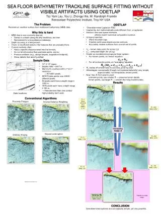
This study presents a novel approach using ODETLAP (Overdetermined Laplacian PDE) for reconstructing seafloor surfaces from multibeam bathymetry (MBB) data. Traditional methods struggle with uneven data spacing and artifacts, leading to inaccurate feature representation. ODETLAP addresses these issues by creating a continuous surface model from sparse data points, optimizing smoothness and accuracy on a pixel-by-pixel basis. Results show significant improvements in mean absolute error compared to conventional algorithms, demonstrating the approach's effectiveness for detailed seafloor mapping.

E N D
SEA FLOOR BATHYMETRY TRACKLINE SURFACE FITTING WITHOUT VISIBLE ARTIFACTS USING ODETLAP Tsz-Yam Lau, You Li, ZhongyiXie, W. Randolph Franklin Rensselaer Polytechnic Institute, Troy NY USA The Problem • Reconstruct seafloor surface from multibeam bathymetry (MBB) data. • Why this is hard • MBB data is very unevenly spaced: • Dense in a swath along the ship tracklines, but then • Nonexistent for a long distance sideways. • Depth accuracy is a few percent. • There is insufficient data to infer features that are probably there. • Current methods often: • Have a specific distance wired into the formula, • Do not let information flow past data points, and so • Produce artifacts (e.g., abrupt slopes, acquisition footprint), • Show details that aren’t justified. • ODETLAP • “OverdeterminedLaplacian PDE” • Inspired by, but mathematically quite different from, a Laplacian. • Solution: time and space intensive, • utilizes recent numerical computation science. • Unique properties: • Infers mountain tops • Creates continuous slopes across contours. • Accurately models surfaces from a small set of points. • hi,j – known data point (for some (i,j)) • zi,j– computed depth (for all (i,j)) • Create an overdetermined sparse linear system: • For known points, an “exact” equation: • zi,j = hi,j • For all nonborder points, an “averaging “equation: • Ri,j (4zi,j = zi-1,j + zi+1,j + zi,j-1 + zi,j+1) • Ri,jtrades off smoothness vs accuracy, pixel by pixel. • Advantages: conceptually (though not implementationally) very simple, • approximates, not interpolates, known points. • New: Vary R from pixel to pixel: • unknown points, use smaller R → preserve terrain details • known points, use larger R → smooth the noisy trackline data. Sample Data • 10oX 10oregion. • Depths: 685 ─ 5917 m. • Want to fit a surface with 0.1°x0.1° resolution • → 601x601 pixels. • 857670 data points over 23630 different pixels. • 54 pixels each have a depth range ≥ 1000 m. • 7878 pixels each have a depth range ≥ 100 m. • → Features less than one contour high probably don’t exist. Results Data locations Conventional Algorithms R= 1 Mean absolute error (MAE): 0.7%* Proximity Polygon Inverse Distance Weighting R= 500 MAE: 6.8%* Increasing FIXED R Second-order spline Ordinary Kriging R= 200 MAE: 5.5%* R= 2 MAE: 1.0%* R= 100 MAE: 4.4%* R= 10 MAE: 2%* Digital picture frame goes here Varying Rs from 10 to 100 MAE: 2.4%* * Relative to data range CONCLUSION Overdetermined systems are conceptually simple, yet very powerful.