Visualizing High-Order Surface Geometry
Explore advanced surface visualization tools to understand the impact of higher-order terms on smooth surfaces. Gain insights into curvature variations, geometric concepts, and fair shape design. Discover the basis for capturing desired effects and optimizing shape functionalities. Unravel open questions on measuring total curvature variation and identifying the most pleasing shape functional. Delve into the analysis of surface curvature in higher dimensions and refine your understanding of 3rd degree surface invariants for intricate surface shapes. Develop a comprehensive perspective on shaping surfaces for optimum aesthetic appeal. Learn to visualize and manipulate complex surface shapes using Fourier coefficients and polynomial height fields. Enhance your grasp of enhancing surface aesthetics through high-order shape bases.

Visualizing High-Order Surface Geometry
E N D
Presentation Transcript
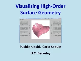
Visualizing High-Order Surface Geometry Pushkar Joshi, Carlo Séquin U.C. Berkeley
Clarification • This talk is NOT about a new CAD tool; but it describes a “Meta-CAD tool.” • This talk is NOT about designing surfaces; it is about understanding smooth surfaces. This Presentation • Convey geometrical insights via a visualization tool for basic surface patches. • Give a thorough understanding of what effects higher-order terms can produce in smooth surfaces.
Visualizing Shape at Surface Point Shape of small patch centered at surface point • Build intuition behind abstract geometric concepts • Applications: differential geometry, smoothness metrics, identifying feature curves on surfaces
Minimizing Curvature Variation for Aesthetic Design Pushkar Joshi, Ph.D. thesis, Oct. 2008 Advisor: Prof. Carlo Séquin U.C. Berkeley http://www.eecs.berkeley.edu/Pubs/TechRpts/2008/EECS-2008-129.html
Minimum Curvature Variation Curves, Networks, and Surfaces for Fair Free-Form Shape Design Henry P. Moreton, Ph.D. thesis, March 1993 Advisor: Prof. Carlo Séquin U.C. Berkeley http://www.eecs.berkeley.edu/Pubs/TechRpts/1993/5219.html
Surface Optimization Functionals MVS optimal shape MVScross optimal shape Minimize: variation of curvature new terms MES optimal shape Minimize: total curvature
Open Questions • What is the right way to measure “total curvature variation” ? • Should one average in-line normal curvature in all directions ? • How many independent 3rd degree terms are there ? • Does MVScross capture all of them, – with the best weighting ? • Gravesen et al. list 18 different 3rd-degree surface invariants ! • How do these functionals influence surface shapes ? • Which functional leads to the fairest, most pleasing shape ? • Which is best basis for capturing all desired effects ? • What is the geometrically simplest way to present that basis ? Draw inspiration from principal curvatures and directions,which succinctly describe second-degree behavior.
Visualizing 2nd Degree Shape Flat Parabolic Hyperbolic Elliptic Principal curvatures (κ1, κ2) and principal directions (e1, e2) completely characterize second-order shape. Can we find similar parameters for higher-order shape?
Understanding the 2nd Degree Terms • Analyze surface curvature in a cylindrical coordinate system centered around the normal vector at the point of interest. • Observe: offset sine-wave behavior of curvature around you, with 2 maxima and 2 minima in the principal directions. Curvature as a function of rotation angle around z-axis: z = n phase-shifted sine-wave: F2plus a constant offset: F0
4 Parameters! Ignore (for now) Polynomial Surface Patch z(u,v) = C0u3 + C1u2v + C2uv2 + C3v3 + Q0u2 + Q1uv + Q2v2 + L0u + L1v + (const.)
Fourier Analysis of Height Field zc(r,θ) = r3[ C0cos3(θ)+ C1cos2(θ)sin(θ)+ C2cos(θ)sin2(θ)+ C3sin3(θ)] zc(r,θ) = r3 [ F1cos( θ + α ) + F3cos(3( θ + α + β )) ] + = F1cos(θ+α) F3cos(3(θ+α+β)) zc(θ)
3rd Degree Shape Basis Components F1 (amplitude) α (phase shift) F3 (amplitude) β (phase shift)
Visualizing 3rd Degree Shape in Fourier Basis F1 component x2 A cubic surface (2 F1 + 2 F3 )/2 = + = F3 component x2
Directions Relevant to 3rd Degree Shape z Maximum F1component Maximum F3component ( 3 equally spaced directions)
GUI of the Visualization Tool Fourier Coefficients PolynomialCoefficients Surface near point of analysis Surface is modified by changing polynomial coefficients or Fourier coefficients. Changing one set of coefficients automatically changes the other set.
Polynomial & Fourier Coefficients z(r, θ) = r3 [ J cos3θ + I sin3θ + H cos2θ sinθ + G cosθ sin2θ ] + r2 [ F cos2θ + E sin2θ + D cosθ sinθ ] + r [ C cosθ + B sinθ ] + A (equivalent) z(r, θ) = r3 [ F3_1cos(θ + α) + F3_3cos3(θ + α + β) ] + r2 [ F2_0 + F2_2cos2(θ + γ) ] + r [ F1_1cos(θ + δ) ] + F0_0 For the math see: Joshi’s PhD thesis
3rd Degree Shape Edits (Sample Sequence) (a) (b) (c) (d) (e) (f)
Visualizing the Properties of a Surface Patch Quadratic overlaid on cubic
Visualizing the Properties of a Surface Patch Arrows indicate significant directions
Visualizing the Properties of a Surface Patch Inline curvature derivative plot
Visualizing the Properties of a Surface Patch Cross curvature derivative plot
3rd Degree Shape Parameters for General Surface Patch κn(θ) κn(θ) (Mehlum-Tarrou 1998) In-line curvature derivative
Recap: 3rd Degree Shape Parameters 2nd Degree: κ1, κ2, φ F0 = (κ1+κ2)/2F2 =(κ1–κ2)/2 3rd Degree: F1, α, F3, βThe F1 and F3 componentsrelate to curvature derivatives.
Higher-Order Shape Bases 4th degree: F0 F2 F4 5th degree: F1 F3 F5
Summary Visualize 3rd degree basis shapes (using polynomial height field) Develop theory of high-order basis shapes (Fourier coefficients) Visualize higher-order (4th degree and 5th degree) basis shapes