Image Enhancement
Image Enhancement. References. Gonzalez and Woods, “ Digital Image Processing,” 2 nd Edition, Prentice Hall, 2002. Jahne, “Digital Image Processing,” 5 th Edition, Springer 2002. Jain, “Fundamentals of Digital Image Processing,” Prentice Hall 1989. Overview.


Image Enhancement
E N D
Presentation Transcript
References • Gonzalez and Woods, “ Digital Image Processing,” 2nd Edition, Prentice Hall, 2002. • Jahne, “Digital Image Processing,” 5th Edition, Springer 2002. • Jain, “Fundamentals of Digital Image Processing,” Prentice Hall 1989
Overview • Human perception (focus of this discussion) • Machine perception (ocr) • Application specific • Heuristic based: result better than the original image – subjective assessment • Spatial vs frequency domain
Spatial Domain • Based on the collection of pixels in the image • Enhancement techniques will yield • Noise reduction • Neighborhood smoothing • Highlighting of desired feature
Spatial Domain – Math Framework From [1] Typically, spatial domain based enhancement involves: g(x,y) = T [f(x,y)], where f = input image; g = output image; T = operator defined on f based on a neighborhood of x,y. If the neighborhood is 1x1 pixel, then the output intensity is dependent on the current intensity value of the pixel, and can be represented as s = T( r )where r and s are gray level values of f(x,y) and g(x,y) at location x,y. In such situations T is a gray-level transformation function.
Examples of Gray level Transformation Functions (Point Processing) From [1] Contrast Stretching Best if input is 0 outside a range of values. Thresholding: Result is a binary Image
Larger Neighborhoods • Objective – determine g(x,y) based on input intensity (gray level) values f(x,y) in the neighborhood of x,y. • Mask processing or filtering • Each of the elements in the neighborhood has an associated weight • g(x,y) depends on f(a,b)|a,b є N(x,y)
Basic Gray Level Transformations Light From [1] Dark Dark Light
Image Negatives From [1] In this example, using the image negative, it is easier to analyze the breast tissue.
Log transformations • s = c log (1 + r) • r >= 0; hence 1 + r > 0; log 0 = ? • Log transformations are useful, when there is a large dynamic range for the input variable ( r ). From [1] Range: 0 to 1.5*106 Range: 0 to 6.2
Power law transformation From [1] Stretch higher (lighter) gray levels Many display devices (e.g. CRT) respond like the power law, i.e intensity – voltage relationship is power law based gamma 1.8 to 2.5. The display will tend to produce images darker than intended. So the display is distorted. Gamma correction is used to correct for this distortion. Stretch lower (ldarker) gray levels
Display distortion correction • Gamma correction can also fix the distortions in color. • More important with the internet. • Many viewers, variety of monitors. • Gamma of view station is not known. • Preprocess using an average gamma. From [1]
Power law – contrast manipulation (c) better than (b). (d) Background is better than (c) but washed out effect. From [1]
Piece-wise Linear Transformation Contrast Stretching From [1] Mean gray level value of the image
Gray level Slicing From [1]
Bit plane Slicing MSb (bit 7) From [1] LSb (bit 0)
Histograms • Histogram - frequency of occurrence of a gray level value • Normalizing histograms with rest to the total number of pixels converts these into probability density like function • Histogram processing yields robust image processing results • Histograms are NOT unique
Histograms for 4 images • For high contrast, it is best to have a larger range of gray level values. • If we could transform an image with a resulting change in histogram, then that may yield more contrast. • We need to study the rules for transforming histograms, and study the resulting impact on images. From [1]
Transformation From [1] s • Applying transformations to histograms, can use results from probability. • Consider the transformation S = T( r ); 0 <= r <=1 which has the following properties: • T( r ) is single-valued and monotonically increasing in [0,1] • 0 <= T( r ) <= 1 for r in [0,1] • Single valued condition ensures that an inverse transformation exists, and the monotonic condition ensures the increasing order of the pixels from black to white. • (a) and (b) do not ensure that the inverse transform is single valued. s1 r r s1 s
Histogram Equalization From [1]
Transformation Functions From [1]
Mapping for Histogram Specification From [1]
Example of Histogram Specification From [1]
Continued From [1]
Localized Histogram Equalization From [1]
Histogram Stats From [1]