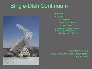
Understanding Single-Dish Continuum Basics and Issues for Future Observing Strategies
Explore the fundamentals, challenges, and strategies in single-dish observations, including gain fluctuations, atmosphere effects, and receiver architectures. Learn about large arrays, thermal emissions, and overcoming confusion limits.

Understanding Single-Dish Continuum Basics and Issues for Future Observing Strategies
E N D
Presentation Transcript
Single-Dish Continuum • Basics • Issues • Confusion • gain fluctuations • atmosphere • Receiver architectures & observing strategies • The future: large arrays Brian Mason (NRAO) NRAO/NAIC Single-Dish Summer School July 13, 2009
ZSPEC (Caltech Submillimeter Observatory) Rotational Transitions Of CO CCH, HCN… Flux Density (Jy) Thermal emission from dust
M82 Stellar death Magnetic fields Thermal BB synchrotron Stellar birth dust Free-Free See Condon (1992, ARA&A)
Dust emission from galaxies at at high redshift • Discovered an abundant population of submm galaxies at z~1-3 • 50 hr map with the JCMT at 850 m, confusion limited HDF-- Hughes et al. (1998)
The Sky Isn’t Empty: Confusion NVSS (45 arcsec FWHM) grayscale GB6 300’ (12 arcmin FWHM) contours
The confusion amplitude P(D) distribution [for n(s) = dN/ds=kS-2.1] Euclidean: D = image brightness (e.g., Jy/beam) Condon (1974); Scheuer (1956)
The confusion amplitude P(D) distribution [for n(s) = dN/ds=kS-2.1] Euclidean: D = 0 mean is not a good baseline; use running median instead Long tail --> use at least 5 sigma threshold (src/30 beams)
The 5σ extragalactic confusion limits forArecibo (d = 220 m) and the GBT (d = 100 m). Gets much weaker with increasing frequency: The noise level won’t go below this if you integrate for longer.
BUT! NRAO VLA Sky Survey (NVSS): 1.4 GHz GB6: old 300’+7-beam receiver, 5 GHz
A Simple Picture of Gain Fluctuations Suppose TSRC << TRX Extra Noise Term (Contributes to baseline ripple for S.L.)
A Simple Picture of Gain Fluctuations DC Offset (e.g., Tsys) Flux Density (Jy)
Why not calibrate the fluctuations away? Stability requirement in order that gain fluctuations cause smaller changes in the output than thermal noise: (1 sec, 1 GHz bw) - too small to be accurately measured each second --> mitigate with instrument design
Atmospheric Emission Sky emission often adds noise to continuum measurements, so you need to measure your noise instead of assuming the radiometer equation or formal uncertainties! How fast do G(t), TATM(t) vary?
Postdetection power spectrum of the receiver output Atmosphere & gain Fluctuations: 1/f Power spectrum Gaussian, uncorrelated Noise (Radiometer Equation): White (flat) power spectrum νk
How does kdepend on bandwidth? νk Less bandwidth νk More bandwidth Eliminate bad fluctuating signals by independently measuring the bad signal on some timescale or shorter. Use < 1/(2πνk): Dicke switching, chopping, multi pixel, etc..
Characteristic Timescales for Broadband Measurements Gain fluct. For coherent amplifiers: 100+ Hz receiver architecture incoherent (bolometer) detectors: 0.1-10 Hz Atmosphere 0.1-few Hz chopping or rapid scanning common mode subtraction for imaging arrays
Dicke-Switching Receiver Rapidly alternate between feed horns to achieve theoretical noise performance. (old-fashioned receiver architecture but good illustration, & same principle as “chopping”) For TSRC<<TSYS gain fluctuations don’t contribute significantly to the noise
Dicke-Switching Receiver Rapidly alternate between feed horns to achieve theoretical noise performance • Penalty: • Differential sky measurement • 2x higher thermal noise
Dicke-Switching Receiver What happens if the feeds see slightly different things? Components before the switch must be as identical + well matched as possible.
An Easier Way? Primarily you switch to suppress receiver effects. Switch must be before active (unstable) components
Correlation Receiver Receiver noise is uncorrelated and drops out. Always looking at both source & reference: only lose one sqrt(2) for differencing
Correlation Polarimeter See talk by Carl Heiles
Higher-Order Differences: Symmetric Nodding • For sensitive photometry, one level of differencing is usually not enough • Gradient in sky emission, or with time • Dual-feed systems: Slight differences in feedhorn gains or losses
Bolometers • Bolometer detectors • Incoherent; measure total power • Very broad bandwidths possible; approach quantum - limited noise. • Can be built in very large-format arrays! MUSTANG (18 GHz)
Bolometers θ MUSTANG (18 GHz) (principle also applies to dual pixel heterodyne receivers & FPAs)
ALFA ALFA on Arecibo 7-element λ = 21 cm coherent array, 3 arcmin resolution GALFACTS:full-Stokes , sensitive, high-resolution survey of 12,000 deg^2 Galactic magnetic fields, ISM, SNR, HII regions, molecular clouds …
Large Format Heterodyne Arrays • QUIET • 91 pixels • I,Q,U • 90 GHz • integrated, mass-producable “receiver on a chip” (MMIC) T. Gaier (JPL)
Large Format Heterodyne Arrays • QUIET • 91 pixels • I,Q,U • 90 GHz • integrated, mass-producable “receiver on a chip” (MMIC) • OCRA • 1-cm Receiver Array • Under construction at Jodrell Bank, initially for Torun 30m telescope • SZ surveys + imaging • 16 --> 100 pixels • correlation architecture T. Gaier (JPL)
Millimeter • ACT (6m) , SPT (10M) • 1-2 mm • Large Area Surveys (SZ) - 1000s of deg^2 • few 1000 detectors • Bolocam/AZTEC • 1-2 mm • 144 pixels • CSO (10m) & LMT (50m) Also IRAM 30m, APEX
Sub-millimeter • SCUBA-2 • JCMT (15m) • ~10,000 pixels! • SQUID-MUX’d TES bolometers (CCD-like) • Under commissioning now Also: SHARC-II on CSO, 384 pixels at 350 um
MUSTANG GBT 3.3mm Bolometer Array Prototype for a 1000-pixel class camera Maping Speed >15x ALMA Thermal Dust + Free-Free Emission In Orion KL/Integral Filament Region.
MUSTANG GBT 3.3mm Bolometer Array Prototype for a 1000-pixel class camera Maping Speed >15x ALMA SZE in RXJ1347-1145 User instruments
Performance Measures From before: Gain An effective aperture of 2760 m2 is required to give a sensitivity of 1.0 K/Jy. Units of 1/Janskys. You sometimes see The System-Equivalent Flux Density, SEFD (small is good) “Mapping Speed” commonly defined as: These are single-pixel measures. For mapping, increase by Nfeeds.
Gain Effects: deviations from linearity Ideal Gain compression/ saturation Output Power TRx Input Power Integrated power is what usually matters (RFI)
Gain Effects: deviations from linearity Ideal Gain compression/ saturation Output Power TRx Input Power Integrated power is what usually matters (RFI) Be aware of the limitations of the instrument You’re using & calibrate at a similar total power Level to what your science observations will see.
Gain Effects: fluctuations Gain drifts over the course of an observing Session(s) easily removed with instrumental Calibrators (e.g., noise diodes) Short term gain fluctuations can be more Problematic. (see continuum lecture)
Sampling/Quantization & Dynamic Range: Postdetection A/D 2N levels (N~14) . . . Diode or square law detector: Turns E-field into some output Proportional to power (E2) Common for continuum systems. Robust & simple (large dynamic range) ~1 level A/D sample time
Sampling/Quantization & Dynamic Range: Predetection Sample the E-field itself. Samplers must be much faster and sample much more corasely (typically just a few levels) Dynamic range limitations more important One usually requires variable attenuators to get it right (“Balancing”). Small # of levels increases the noise level. (K-factor in Radiometer equation) More levels -> greater dynamic range (RFI robustness), greater sensitivity Monitor levels through your observation.
Nonthermal Emission around Sgr A* 75 MHz, VLA: 330 MHz, GBT: LaRosa, Brogan et al. (2005)