Linear algebra: matrices
Linear algebra: matrices. Horacio Rodríguez. Introduction. Some of the slides are reused from my course on graph-based methods in NLP (U. Alicante, 2008) http://www.lsi.upc.es/~horacio/varios/graph.tar.gz so, some of the slides are in Spanish

Linear algebra: matrices
E N D
Presentation Transcript
Linear algebra: matrices Horacio Rodríguez
Introduction • Some of the slides are reused from my course on graph-based methods in NLP (U. Alicante, 2008) • http://www.lsi.upc.es/~horacio/varios/graph.tar.gz • so, some of the slides are in Spanish • Material can be obtained from wikipedia (under the articles on matrices, linear algebra, ...) • Another interesting source is Wolfram MathWorld • (http://mathworld.wolfram.com) • Several mathematical software packages provide implementation of the matrix operations and decompositions: • Matlab (I have tested some features) • Mapple • Mathematica
Vectorial Spaces • Vectorial Spaces • dimension • Bases • Sub-spaces • Kernel • Image • Linear maps • Ortogonal base • Metric Spaces • Ortonormal base • Matrix representation of a Linear map • Basic operations on matrices
Basic concepts • Matriz hermítica (autoadjunta) • A = A* , A es igual a la conjugada de su traspuesta • Una matriz real y simétrica es hermítica • A* = AT • Una matriz hermítica es normal • Todos los valores propios son reales • Los vectores propios correspondientes a valores propios distintos son ortogonales • Es posible encontrar una base compuesta sólo por vectores propios • Matriz normal • A*A = AA* • si A es real, ATA = AAT • Matriz unitaria • A*A = AA* = In • si A es real, A unitaria ortogonal
Transpose of a matrix • The transpose of a matrix A is another matrix AT created by any one of the following equivalent actions: • write the rows of A as the columns of AT • write the columns of A as the rows of AT • reflect A by its main diagonal (which starts from the top left) to obtain AT
Positive definite matrix • For complex matrices, a positive-definite matrix is a (Hermitian) matrix if z*Mz > 0 for all non-zero complex vectors z. The quantity z*Mz is always real because M is a Hermitian matrix. • For real matrices, an n × n real symmetric matrix M is positive definite if zTMz > 0 for all non-zero vectors z with real entries (i.e. z ∈ Rn). • A Hermitian (or symmetric) matrix is positive-definite iff all its eigenvalues are > 0.
Bloc decomposition • Algunos conceptos a recordar de Álgebra Matricial • Descomposición de una matriz en bloques • bloques rectangulares
Bloc decomposition • Descomposición de una matriz en bloques • Suma directa A B, A m n, B p q • Block diagonal matrices (cuadradas)
Matrix decomposition • Different decompositions are used to implement efficient matrix algorithms.. • For instance, when solving a system of linear equations Ax = b, the matrix A can be decomposed via the LU decomposition. The LU decomposition factorizes a matrix into a lower triangular matrix L and an upper triangular matrix U. The systems L(Ux) = b and Ux = L− 1b are much easier to solve than the original. • Matrix decomposition at wikipedia: • Decompositions related to solving systems of linear equations • Decompositions based on eigenvalues and related concepts
LU decomposition • Descomposiciones de matrices • LU • A matriz cuadrada compleja n n • A = LU • L lower triangular • U upper triangular • LDU • A = LDU • L unit lower triangular (las entradas de la diagonal son 1) • U unit upper triangular (las entradas de la diagonal son 1) • D matriz diagonal • LUP • A = LUP • L lower triangular • U upper triangular • P matriz permutación • sólo 0 ó 1 con un solo 1 en cada fila y columna
LU decomposition • Existence • An LUP decomposition exists for any square matrix A • When P is an identity matrix, the LUP decomposition reduces to the LU decomposition. • If the LU decomposition exists, the LDU decomposition does too. • Applications • The LUP and LU decompositions are useful in solving an n-by-n system of linear equations Ax = b
Cholesky decomposition • Descomposiciones de matrices • Cholesky • A hermítica, definida positiva • y, por lo tanto, a matrices cuadradas,reales, simétricas, definidas positivas • A = LL* o equivalentemente A = U*U • L lower triangular con entradas en la diagonal estrictamente positivas • the Cholesky decomposition is a special case of the symmetric LU decomposition, with L = U* (or U=L*). • the Cholesky decomposition is unique
Cholesky decomposition • Cholesky decomposition in Matlab • A must be positive definite; otherwise, MATLAB displays an error message. • Both full and sparse matrices are allowed • syntax • R = chol(A) • L = chol(A,'lower') • [R,p] = chol(A) • [L,p] = chol(A,'lower') • [R,p,S] = chol(A) • [R,p,s] = chol(A,'vector') • [L,p,s] = chol(A,'lower','vector')
Cholesky decomposition • Example • The binomial coefficients arranged in a symmetric array create an interesting positive definite matrix. • n = 5 • X = pascal(n) • X = • 1 1 1 1 1 • 1 2 3 4 5 • 1 3 6 10 15 • 1 4 10 20 35 • 1 5 15 35 70
Cholesky decomposition • Example • It is interesting because its Cholesky factor consists of the same coefficients, arranged in an upper triangular matrix. • R = chol(X) • R = • 1 1 1 1 1 • 0 1 2 3 4 • 0 0 1 3 6 • 0 0 0 1 4 • 0 0 0 0 1
Cholesky decomposition • Example • Destroy the positive definiteness by subtracting 1 from the last element. • X(n,n) = X(n,n)-1 • X = • 1 1 1 1 1 • 1 2 3 4 5 • 1 3 6 10 15 • 1 4 10 20 35 • 1 5 15 35 69 • Now an attempt to find the Cholesky factorization fails.
QR decomposition • QR • A real matrix m n • A = QR • R upper triangular m n • Q ortogonal (QQT = I) m m • similarmente • QL • RQ • LQ • Si A es no singular (invertible) la factorización es única si los elementos de la diagonal principal de R han de ser positivos • Proceso de ortonormalización de Gram-Schmidt
QR decomposition • QR in matlab: • Syntax • [Q,R] = qr(A) (full and sparse matrices) • [Q,R] = qr(A,0) (full and sparse matrices) • [Q,R,E] = qr(A) (full matrices) • [Q,R,E] = qr(A,0) (full matrices) • X = qr(A) (full matrices) • R = qr(A) (sparse matrices) • [C,R] = qr(A,B) (sparse matrices) • R = qr(A,0) (sparse matrices) • [C,R] = qr(A,B,0) (sparse matrices)
QR decomposition • example: • A = [1 2 3 • 4 5 6 • 7 8 9 • 10 11 12 ] • This is a rank-deficient matrix; the middle column is the average of the other two columns. The rank deficiency is revealed by the factorization: • [Q,R] = qr(A) • Q = • -0.0776 -0.8331 0.5444 0.0605 • -0.3105 -0.4512 -0.7709 0.3251 • -0.5433 -0.0694 -0.0913 -0.8317 • -0.7762 0.3124 0.3178 0.4461 • R = • -12.8841 -14.5916 -16.2992 • 0 -1.0413 -2.0826 • 0 0 0.0000 • 0 0 0 • The triangular structure of R gives it zeros below the diagonal; the zero on the diagonal in R(3,3) implies that R, and consequently A, does not have full rank.
Projection • Proyección • P tal que P2 = P (idempotente) • Una proyección proyecta el espacio W sobre un subespacio U y deja los puntos del subespacio inalterados • x U, rango de la proyección: Px = x • x V, espacio nulo de la proyección: Px = 0 • W = U V, U y V son complementarios • Los únicos valores propios son 0 y 1, W0 = V, W1 = U • Proyecciones ortogonales: U y V son ortogonales
Centering matrix • matriz simétrica e idempotente que multiplicada por un vector tiene el mismo efecto que restar a cada componente del vector la media de sus componentes • In matriz identidad de tamaño n • 1 vector columna de n unos • Cn = In -1/n 11T
Eigendecomposition • especial case of linear map areendomorphisms • i.e. maps f: V → V. • In this case, vectors v can be compared to their image under f, f(v). Any vector v satisfying λ · v = f(v), where λ is a scalar, is called an eigenvector of f with eigenvalue λ • v is an element of kernel of the difference f − λ · I • In the finite-dimensional case, this can be rephrased using determinants • f having eigenvalue λ is the same as det (f − λ · I) = 0 • characteristic polynomial of f • The vector space V may or may not possess an eigenbasis, i.e. a basis consisting of eigenvectors. This phenomenon is governed by the Jordan canonical form of the map. • The spectral theorem describes the infinite-dimensional case
Eigendecomposition • Decomposition of a matrix A into eigenvalues and eigenvectors • Each eigenvalue is paired with its corresponding eigenvector • This decomposition is often named matrix diagonalization • nondegenerate eigenvalues 1 ...n • D is the diagonal matrix formed with the set of eigenvalues • linearly independent eigenvectors X1 ... Xn • P is the matrix formed with the columns corresponding to the set of eigenvectors • AX = X • if the n eigenvalues are distinct, P is invertible • A = PDP-1
Eigendecomposition • Teorema espectral • condiciones para que una matriz sea diagonalizable • A matriz hermítica en un espacio V (complejo o real) dotado de un producto interior • <Ax|y> = <x|Ay> • Existe una base ortonormal de V consistente en vectores propios de A. Los valores propios son reales • Descomposición espectral de A • para cada valor propio diferente V={vV: Av=v} • V es la suma directa de los V • Diagonalización • si A es normal (y por tanto si es hermítica y por tanto si es real simétrica) entonces existe una descomposición • A = U U* • es diagonal, sus entradas son los valores propios de A • U es unitaria, sus columnas son los vectores propios de A
Eigendecomposition • Caso de matrices no simétricas • rk right eigenvectors Ark = rk • lk left eigenvectors lkA = lk • Si A es real • ATlk= lk • Si A es simétrica • rk = lk
Eigendecomposition • Eigendecomposition in Matlab • Syntax • d = eig(A) • d = eig(A,B) • [V,D] = eig(A) • [V,D] = eig(A,'nobalance') • [V,D] = eig(A,B) • [V,D] = eig(A,B,flag)
Jordan Normal Form • Jordan normal form • una matriz cuadrada A n n es diagonalizable ssi la suma de las dimensiones de sus espacios propios es n tiene n vectores propios linealmente independientes • No todas las matrices son diagonalizables • dada A existe siempre una matriz P invertible tal que • A = PJP-1 • J tiene entradas no nulas sólo en la diagonal principal y la diagonal superior • J está en forma normal de Jordan
Jordan Normal Form • Example • Consider the following matrix: • The characteristic polynomial of A is: • eigenvalues are 1, 2, 4 and 4 • The eigenspace corresponding to the eigenvalue 1 can be found by solving the equation Av = v. So, the geometric multiplicity (i.e. dimension of the eigenspace of the given eigenvalue) of each of the three eigenvalues is one. Therefore, the two eigenvalues equal to 4 correspond to a single Jordan block,
Jordan Normal Form • Example • The Jordan normal form of the matrix A is the direct sum of the three Jordan blocs • The matrix J is almost diagonal. This is the Jordan normal form of A.
Schur Normal Form • Descomposiciones de matrices • Schur • A matriz cuadrada compleja n n • A = QUQ* • Q unitaria • Q* traspuesta conjugada de Q • U upper triangular • Las entradas de la diagonal de U son los valores propios de A
SVD • Descomposiciones de matrices • SVD • Generalización del teorema espectral • M matriz m n • M = U V* • U m m unitary ortonormal input • V n n unitary ortonormal output • V* transpuesta conjugada de V • matriz diagonal con entradas no negativas valores propios • Mv = u, M*u = v, valor propio, u left singular vector, v right singular vector • Las columnas de U son los vectores propios u • Las columnas de V son los vectores propios v • Aplicación a la reducción de la dimensionalidad • Principal Components Analysis