Download
1 / 25
250 likes | 272 Vues
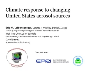
Climate response to changing United States aerosol sources. Eric M. Leibensperger , Loretta J. Mickley, Daniel J. Jacob School of Engineering and Applied Sciences, Harvard University. Wei-Ting Chen, John Seinfeld Department of Environmental Science and Engineering, Caltech. David Streets

E N D
Climate response to changing United States aerosol sources Eric M. Leibensperger, Loretta J. Mickley, Daniel J. Jacob School of Engineering and Applied Sciences, Harvard University Wei-Ting Chen, John Seinfeld Department of Environmental Science and Engineering, Caltech David Streets Argonne National Laboratory Support from:
Climate Change Affects Air Quality Mid-latitude cyclones can act as an explantory variable for air pollution episodes The frequency of cyclones tracking through the southern climatological storm track is strongly anti-correlated with the number of ozone exceedances. Cyclones summarize meteorological parameters driving ozone changes: temperature, humidity, sunshine and ventilation. [Leibensperger, 2008]
O3 Controls Have Not Realized Their Full Potential Observations and assimilated meteorology show comparable trends in the number of cyclones (-0.15 a-1 vs. -0.14 a-1). The end result is the same - the trend derived due to emissions alone would have reached an expected value of zero by 2001 in the absence of a trend of mid-latitude cyclones. [Leibensperger, 2008]
Short-lived Pollutants Affect Climate and Air Quality [IPCC, 2007] Regulations of short-lived species that improve air quality and warm the planet (BC) present a “win-win” situation, while regulations of short-lived species that reduce cooling and improve air quality (SO2) present a “win-lose” situation.
Climate Effects of Changes in Aerosols & Ozone Do aerosols and ozone, which are not well-mixed in the atmosphere, have climate effects that match their spatial distribution or more global in scale? [Mickley et a, in prep.] [Shindell, 2008]
Changing Air Quality and Climate in the U.S. The US has had and is expected to have large changes in aerosol and ozone precursor emissions. How do the changes in these air pollutants affect the climate of the United States? Surface Solar Radiation (W/m2) 1981-1990 1971-1980 1961-1970 [Liepert, 2002] 4th Highest Daily Mean 8-Hr Concentration Month [EPA, 2008]
Modeling Framework: From Emissions to Climate Past, Present, Future Emissions GEOS-Chem chemical transport model BC, POA, SOA, (NH4)2SO4, (NH4)NO3, Aerosol H2O, Sea Salt GISS GCM 3climate model Sensitivity simulations with GEOS-Chem and the GISS GCM allow us to quantify the impact of U.S. emissions on regional and global climate
From Emissions to 3-D Concentrations: GEOS-Chem • Chemical Transport Model: • GEOS-Chem v8-01-01 • 2o x 2.5o resolution • GEOS-4 meteorology for 2001 – precludes climate’s influence on aerosols • MARS-A aerosol thermodynamic equilibrium model • Two year simulations were conducted for each decade (1950, 1960…2050), the first being used as spin-up. 1950 2010 2050 Control - Reconstructed Emissions and A1B 0 U.S. SO2, NOx, BC and POA Emissions
Past, Present, and Future Emissions EDGAR (SO2, NOx) Bond 2007 (BC, OC) A1B Regional Scale Factors from Streets 2004 Emissions from biomass burning, NH3, CO, and other trace gases held constant at present day levels.
Model Evaluation: Sulfate, Nitrate, Ammonium The model compares favorably with observed concentrations of sulfate, nitrate, and ammonium, capturing the spatial gradients and industrial “hot spots.” Sulfate and ammonium match the magnitude of the observations very well, while nitrate is underestimated in the Midwest.
Model Evaluation: Black Carbon and Organic Carbon The model generally has a low bias of BC compared to IMPROVE observations. The bias is likely due to the lower emissions of BC we use from Bond et al. [2007]. The model captures the magnitude and spatial gradient of much of the OC observations.
Further Model Evaluation: Wet Deposition The model is able to capture the spatial distribution and magnitude of annual wet deposition. The species shown here are all pretty soluble. As a result this is more a test of emissions than chemistry. Ammonia is too low over the Midwest, explaining the model’s low nitrate concentrations and deposition.
Further Model Evaluation: Wet Deposition (2) Sulfate Nitrate Ammonium The longer time series of wet deposition data allows for the comparison of emissions of earlier decades. Note the success of total ammonium deposition throughout the decades, despite using constant emissions throughout.
Global Aerosol Burdens The US has influenced the amount of sulfate in the global atmosphere more than the other species. Removing the US source of SO2 has the effect of slightly increasing the amount of aerosol nitrate due to an increase in the amount of available ammonia. This effect disappears as global sources of SO2 become larger. By 2050, in the A1B scenario, the US-sourced aerosol are a small fraction of the global burden.
Aerosol Burdens over the United States The US is increasingly influenced by foreign sources. In the future, sulfate, BC, and OC over the US decrease due to emission reductions. Aerosol nitrate levels off and slightly increases even though NOx emissions continue to fall. With no US anthropogenic sources, sulfate increases due to changes in foreign sources of SO2.
PM2.5 Enhancement from U.S. Aerosol Sources U.S. aerosol sources enhance aerosol formation over the U.S. and its outflow region. Through changes in oxidant concentrations, the U.S. additionally affects downstream aerosol amounts (0.5 μg m-3 in DJF). The downwind effects are localized due to high emissions of SO2, NOx, and ammonia.
AOD Enhancement from U.S. Aerosol Sources (2) The global influence of the US on AOD increases from 1950 to 1990. From 1950 to 2040, the AOD over the US is increasing due to external increases in SO2 and NOx emissions.
Radiative Forcing from Anthropogenic Aerosol Internal mixing increases the ability of BC to absorb solar radiation, reducing the TOA radiative forcing.
Radiative Forcing from U.S. Sources Similar to the sulfate burden, radiative forcing over the eastern US maximizes in the 1980-90s and begins a steep decrease.
From 3-D Concentrations to Climate Changes: GISS GCM 3 • Global Climate Model: • GISS GCM 3 • 4o x 5o resolution • Q-Flux ocean representation • With modifications to tropospheric aerosol interface from Caltech [Chen et al., accepted] • Transient climate simulations were begun in 1950 and continued until 2050. • Ensembles of four control and four sensitivity simulations were compared • All results shown have 95% significance. 1950 2010 2050 Control - Reconstructed Emissions and A1B 0 U.S. SO2, NOx, BC and POA Emissions
Change in Present Day Annual Mean Surface Temperature U.S.-sourced aerosol sources have cooled the annual mean surface temperature of the eastern U.S. by 0.5-0.75°C What’s plotted: Control – No US Aerosol Sources
Change in Temperature due to U.S. Aerosols: 1950-2050 ΔT The temperature response over the U.S. does not match the TOA radiative forcing time series calculated “offline.” For much of the time period considered, the temperature change due to U.S.-sourced aerosols is relatively constant, like the surface forcing due to compensating trends in sulfate and BC. What’s plotted: Control – No US Aerosol Sources
What causes the temperature response to differ from the RF? Changes in cloud cover, solar radiation, TOA net solar radiation, and cloud cover all correlate well with changes in surface air temperature. There are likely feedbacks acting that regulate the response.
Other Changes Due to U.S. Aerosols - JJA A persistent change due to U.S.-sourced aerosols is the reduction of evaporation off of the East Coast and resulting reduction in precipitation. Changes in latent heat flux, along with changes in baroclinicity, are potential mechanisms to “broadcast” the climate signal.
What is next? • Analyze daily data. • Complete control simulations that omit US BC. This will help us clarify the role that BC is playing in the changes we are seeing. • Incorporate the indirect aerosol effects using the implementation of the 1st and 2nd indirect aerosol effects to the GISS GCM 3 by Caltech (Chen et al., in press). • Further analysis of the effects of the changing mix of US-sources aerosols (e.g. decreasing BC while sulfate increases) THANKS!! Eric Leibensperger – eleibens@fas.harvard.edu